A class of finite dimensional spaces and H(div) conformal elements on general polytopes
Pith reviewed 2026-05-24 18:54 UTC · model grok-4.3
The pith
H(div)-conformal finite element spaces can be built on arbitrary polytopes while preserving Raviart-Thomas divergence properties at every interface.
A machine-rendered reading of the paper's core claim, the machinery that carries it, and where it could break.
Core claim
We present a class of discretisation spaces and H(div)-conformal elements that can be built on any polytope. Bridging the flexibility of the Virtual Element spaces towards the element's shape with the divergence properties of the Raviart-Thomas elements on the boundaries, the designed frameworks offer a wide range of H(div)-conformal discretisations. As those elements are set up through degrees of freedom, their definitions are easily amenable to the properties the approximated quantities are wished to fulfil. Furthermore, we show that one straightforward restriction of this general setting share its properties with the classical Raviart-Thomas elements at each interface, for any order and任何
What carries the argument
The construction of the spaces via boundary degrees of freedom chosen to enforce H(div) conformity while retaining Raviart-Thomas divergence behavior on every face of an arbitrary polytope.
If this is right
- The spaces can be used on meshes composed of arbitrary polytopes without loss of H(div) conformity.
- The Raviart-Thomas interface properties hold for every polynomial degree and every polytope shape.
- The degree-of-freedom definition allows the spaces to be tailored to additional properties required by the target problem.
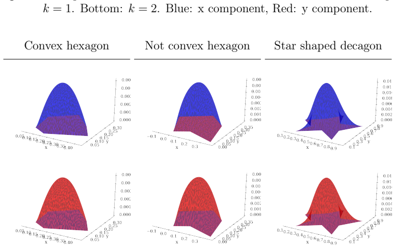
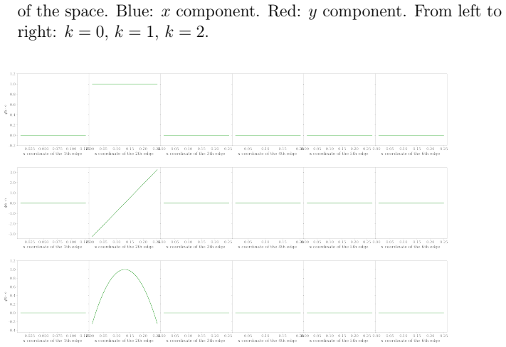
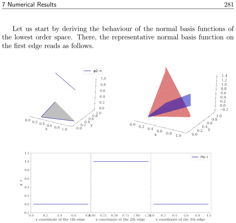
- Basis functions for the resulting elements can be explicitly studied in two dimensions.
Where Pith is reading between the lines
- The same boundary-degree-of-freedom strategy might be adapted to produce H(curl)-conforming spaces on general polytopes.
- Meshes generated from arbitrary polyhedral decompositions of complex domains become directly usable without additional conformity fixes.
- Hybrid discretizations that mix these elements with standard Raviart-Thomas elements on selected faces become feasible.
Load-bearing premise
It is possible to choose degrees of freedom on the boundaries of arbitrary polytopes so that the spaces remain H(div)-conforming and keep the divergence properties of Raviart-Thomas elements.
What would settle it
A concrete counter-example in which the normal traces of the constructed vector fields fail to be continuous across an interface between two non-convex polytopes of the same polynomial order.
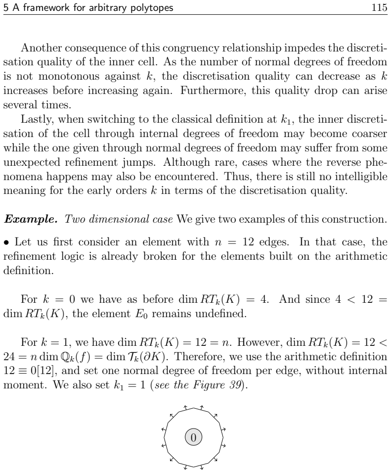
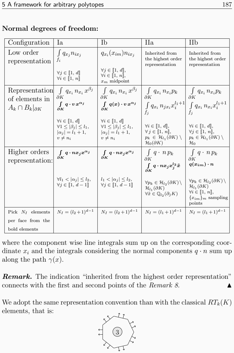
Figures


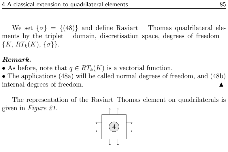


read the original abstract
We present a class of discretisation spaces and H(div)-conformal elements that can be built on any polytope. Bridging the flexibility of the Virtual Element spaces towards the element's shape with the divergence properties of the Raviart-Thomas elements on the boundaries, the designed frameworks offer a wide range of H(div)-conformal discretisations. As those elements are set up through degrees of freedom, their definitions are easily amenable to the properties the approximated quantities are wished to fulfil. Furthermore, we show that one straightforward restriction of this general setting share its properties with the classical Raviart-Thomas elements at each interface, for any order and any polytopial shape. Then, we investigate the shape of the basis functions corresponding to particular elements in the two dimensional case.
Editorial analysis
A structured set of objections, weighed in public.
Referee Report
Summary. The manuscript introduces a general class of finite-dimensional spaces and H(div)-conforming finite elements on arbitrary polytopes, combining the shape flexibility of Virtual Element Methods with the divergence properties of Raviart-Thomas elements on element boundaries. The spaces are defined via degrees of freedom, and the central result is that one straightforward restriction of the general construction reproduces the interface properties of classical Raviart-Thomas elements (normal traces and exact divergence mapping) for any polynomial order and any polytope shape. The paper also examines the geometry of basis functions in the two-dimensional case.
Significance. If the H(div)-conformity, normal continuity, and exact-sequence properties are established without hidden geometric restrictions on the polytopes, the framework would enable mixed finite-element discretizations on completely general polyhedral meshes. This flexibility is potentially useful for applications such as Darcy flow or incompressible elasticity on unstructured grids. The DOF-based definition is a methodological strength that facilitates adaptation to additional constraints.
major comments (1)
- [Abstract and section describing the construction of the spaces] Abstract / construction of the spaces: The claim that a restriction of the general setting reproduces the classical Raviart-Thomas normal traces and the exact div(P_k) property on every interface, for arbitrary polytopes and any order, rests on an unverified choice of face degrees of freedom. The manuscript must supply the explicit definition of these boundary DOFs together with the algebraic argument showing that they simultaneously enforce normal continuity, lie in the RT trace space, and preserve the surjectivity of the divergence operator onto the full polynomial space inside the element, without additional hypotheses (e.g., star-shapedness or convexity of the polytope or its faces).
minor comments (1)
- [Abstract] The sentence 'one straightforward restriction of this general setting share its properties' contains a subject-verb agreement error and should read 'shares its properties'.
Simulated Author's Rebuttal
We thank the referee for the thorough review and for highlighting the need for greater explicitness in the construction of the restricted spaces. We address the single major comment below and will incorporate the requested clarifications in a revised manuscript.
read point-by-point responses
-
Referee: [Abstract and section describing the construction of the spaces] Abstract / construction of the spaces: The claim that a restriction of the general setting reproduces the classical Raviart-Thomas normal traces and the exact div(P_k) property on every interface, for arbitrary polytopes and any order, rests on an unverified choice of face degrees of freedom. The manuscript must supply the explicit definition of these boundary DOFs together with the algebraic argument showing that they simultaneously enforce normal continuity, lie in the RT trace space, and preserve the surjectivity of the divergence operator onto the full polynomial space inside the element, without additional hypotheses (e.g., star-shapedness or convexity of the polytope or its faces).
Authors: We agree that the original manuscript presented the restricted construction at a high level and did not spell out the face degrees of freedom or the accompanying algebraic verification in sufficient detail. In the revised version we will add an explicit subsection that defines the boundary degrees of freedom of the restricted space as the standard Raviart-Thomas moments ∫_f (v·n) q ds for all q ∈ P_k(f) on each face f. We will then supply a self-contained algebraic argument showing that these moments (i) force the normal trace on each face to lie in the RT trace space P_k(f), (ii) guarantee normal continuity across interfaces because adjacent elements share identical face moments, and (iii) preserve surjectivity of the divergence onto the full P_k inside the element by a dimension-counting argument that uses only the exact polynomial sequence on the boundary and the complementary internal degrees of freedom. The argument relies exclusively on the unisolvence of the chosen degrees of freedom and the algebraic properties of the polynomial spaces; it invokes no geometric hypotheses such as star-shapedness or convexity of the polytope or its faces. revision: yes
Circularity Check
No circularity: construction presented as independent of its target properties
full rationale
The abstract and description present a general class of spaces defined via degrees of freedom on polytopes, with a restriction to Raviart-Thomas-like behavior stated as a result that is shown rather than presupposed by definition. No equations, fitted parameters renamed as predictions, or self-citation chains appear in the provided text. The derivation is therefore treated as self-contained against external finite-element theory.
Axiom & Free-Parameter Ledger
Reference graph
Works this paper leans on
-
[1]
R. Abgrall, E. le M´ el´ edo, and P. ¨Offner. On the Connection be- tween Residual Distribution Schemes and Flux Reconstruction. https: //arxiv.org/abs/1807.01261, July 2018
-
[2]
D. Boffi, F. Brezzi, M. Fortin, et al. Mixed finite element methods and applications, volume 44. Springer, 2013
work page 2013
- [3]
-
[4]
F. Brezzi and M. Fortin, editors. Mixed and Hybrid Finite Element Methods. Springer New York, 1991
work page 1991
-
[5]
J. Chabrowski. The Dirichlet problem with L2-boundary data for elliptic linear equations. Springer, 2006
work page 2006
-
[6]
B. Cockburn, G. E. Karniadakis, and C.-W. Shu. Discontinuous Galerkin methods: theory, computation and applications , volume 11. Springer Science & Business Media, 2012
work page 2012
-
[7]
D. A. Di Pietro and S. Lemaire. An extension of the Crouzeix-Raviart space to general meshes with application to quasi-incompressible linear elasticity and Stokes flow. Mathematics of Computation , 84(291):1–31, 2015
work page 2015
-
[8]
Raviart-Thomas finite elements of Petrov-Galerkin type
F. Dubois, I. Greff, and C. Pierre. Raviart-thomas finite elements of petrov-galerkin type. arXiv preprint arXiv:1710.04395 , 2017
work page internal anchor Pith review Pith/arXiv arXiv 2017
-
[9]
V. Ervin. Computational bases for rtk and bdmk on triangles. Comput- ers & Mathematics with Applications , 64(8):2765–2774, 2012
work page 2012
-
[10]
A. Gillette, A. Rand, and C. Bajaj. Construction of scalar and vector finite element families on polygonal and polyhedral meshes
-
[11]
J. Gopalakrishnan, L. E. Garc´ ıa-Castillo, and L. F. Demkowicz. N´ ed´ elec spaces in affine coordinates. Computers & Mathematics with Applica- tions, 49(7-8):1285–1294, 2005
work page 2005
-
[12]
H. T. Huynh. A flux reconstruction approach to high-order schemes including discontinuous galerkin methods. In 18th AIAA Computational Fluid Dynamics Conference, page 4079, 2007. B Details of some elements used in the numerical experiments 310
work page 2007
-
[13]
J.C. N´ ed´ elec. Mixed finite elements in R3. Numerische Mathematik , 35(3):315–341, 1980
work page 1980
-
[14]
M. V. Kondratieva, A. B. Levin, A. V. Mikhalev, and E. V. Pankratiev. Differential and Difference Dimension Polynomials . Springer Nether- lands, 1999
work page 1999
-
[15]
H. Ranocha, P. ¨Offner, and T. Sonar. Summation-by-parts operators for correction procedure via reconstruction. Journal of Computational Physics, 311:299–328, 2016
work page 2016
-
[16]
P. A. Raviart and J. M. Thomas. A mixed finite element method for 2-nd order elliptic problems. In I. Galligani and E. Magenes, editors, Mathematical Aspects of Finite Element Methods, pages 292–315, Berlin, Heidelberg, 1977. Springer Berlin Heidelberg
work page 1977
-
[17]
N. Sukumar and E. Malsch. Recent advances in the construction of polygonal finite element interpolants. Archives of Computational Meth- ods in Engineering, 13(1):129, 2006
work page 2006
-
[18]
C. Talischi, A. Pereira, G. H. Paulino, I. F. Menezes, and M. S. Carvalho. Polygonal finite elements for incompressible fluid flow. International Journal for Numerical Methods in Fluids , 74(2):134–151, oct 2013
work page 2013
-
[19]
J.-M. Thomas. M´ ethode des ´ el´ ements finis hybrides duaux pour les probl` emes elliptiques du second ordre. Revue fran¸ caise d’automatique, informatique, recherche op´ erationnelle. Analyse num´ erique, 10(R3):51– 79, 1976
work page 1976
-
[20]
L. B. D. Veiga, F. Brezzi, A. Cangiani, G. Manzini, L. D. Marini, and A. Russo. Basic principles of virtual element methods. Mathematical Models and Methods in Applied Sciences , 23(01):199–214, jan 2013
work page 2013
-
[21]
P. E. Vincent, P. Castonguay, and A. Jameson. A new class of high- order energy stable flux reconstruction schemes. Journal of Scientific Computing, 47(1):50–72, 2011
work page 2011
discussion (0)
Sign in with ORCID, Apple, or X to comment. Anyone can read and Pith papers without signing in.