When is cumulative dose response monotonic? Analysis of incoherent feedforward motifs
Pith reviewed 2026-05-19 17:42 UTC · model grok-4.3
The pith
Cumulative dose responses stay monotone in most incoherent feedforward motifs even when instantaneous responses do not.
A machine-rendered reading of the paper's core claim, the machinery that carries it, and where it could break.
Core claim
For systems with linear intermediate dynamics and nonlinear output dynamics, an integral representation of cDR sensitivity shows that IFFM1 and IFFM3 exhibit monotone cDR despite potentially non-monotone DR, IFFM2 is monotone already at the DR level, and IFFM4 violates the conditions and loses monotonicity in cDR.
What carries the argument
The integral representation of the sensitivity of the cumulative dose response with respect to the input, which reduces the monotonicity question to verifying qualitative sign properties along system trajectories.
Load-bearing premise
The derivation assumes linear dynamics for the intermediate layer together with nonlinear output dynamics and structured initial conditions.
What would settle it
A numerical trajectory or parameter choice for IFFM1 in which the cumulative dose response decreases as the input increases would falsify the claimed monotonicity.
Figures


read the original abstract
We study the monotonicity of the cumulative dose response (cDR) for a class of incoherent feedforward motifs (IFFM) systems with linear intermediate dynamics and nonlinear output dynamics. While the instantaneous dose response (DR) may be nonmonotone with respect to the input, the cDR can still be monotone. To analyze this phenomenon, we derive an integral representation of the sensitivity of cDR with respect to the input and establish general sufficient conditions for both monotonicity and non-monotonicity. These results reduce the problem to verifying qualitative sign properties along system trajectories. We apply this framework to four canonical IFFM systems and obtain a complete characterization of their behavior. In particular, IFFM1 and IFFM3 exhibit monotone cDR despite potentially non-monotone DR, while IFFM2 is monotone already at the level of DR, which implies monotonicity of cDR. In contrast, IFFM4 violates these conditions, leading to a loss of monotonicity. Numerical simulations indicate that these properties persist beyond the structured initial conditions used in the analysis. Overall, our results provide a unified framework for understanding how network structure governs monotonicity in cumulative input-output responses.
Editorial analysis
A structured set of objections, weighed in public.
Referee Report
Summary. The manuscript analyzes monotonicity of the cumulative dose response (cDR) in incoherent feedforward motif (IFFM) systems with linear intermediate dynamics and nonlinear output dynamics. It derives an integral representation of cDR sensitivity to the input and reduces monotonicity questions to verifying qualitative sign properties along trajectories. The framework is applied to four canonical IFFMs, yielding a characterization: IFFM1 and IFFM3 exhibit monotone cDR despite possibly non-monotone instantaneous dose response (DR); IFFM2 is already monotone at the DR level; IFFM4 violates the sign conditions and loses monotonicity. Numerical simulations suggest the properties persist for other initial conditions.
Significance. If the central claims hold, the work supplies a useful reduction of cDR monotonicity to trajectory sign conditions, offering insight into how motif structure controls cumulative input-output behavior. This is relevant to dynamical systems and systems biology. Strengths include the explicit application to four motifs with a complete characterization, the integral representation approach, and the provision of numerical support for robustness beyond the analytic assumptions.
major comments (1)
- [Derivation of integral representation and application to the four IFFMs] The analytic derivation of the integral representation of cDR sensitivity and the subsequent sign conditions (used to conclude monotonicity for IFFM1 and IFFM3 and loss for IFFM4) are obtained under linear intermediate dynamics together with structured initial conditions. This assumption is load-bearing for the claimed complete characterization, as the abstract notes only that numerics suggest persistence for other conditions without providing an analytic extension or robustness proof for arbitrary ICs or nonlinear intermediates.
minor comments (1)
- Clarify in the abstract and introduction the precise scope of the analytic results versus the numerical evidence.
Simulated Author's Rebuttal
We thank the referee for their careful reading, positive assessment of the work's significance, and constructive feedback on the scope of our analytic results. We address the major comment below and will make targeted revisions to improve clarity.
read point-by-point responses
-
Referee: The analytic derivation of the integral representation of cDR sensitivity and the subsequent sign conditions (used to conclude monotonicity for IFFM1 and IFFM3 and loss for IFFM4) are obtained under linear intermediate dynamics together with structured initial conditions. This assumption is load-bearing for the claimed complete characterization, as the abstract notes only that numerics suggest persistence for other conditions without providing an analytic extension or robustness proof for arbitrary ICs or nonlinear intermediates.
Authors: We agree that the integral representation of cDR sensitivity and the resulting sign conditions for monotonicity are derived under the assumptions of linear intermediate dynamics and structured initial conditions, as stated in the manuscript (see Section 2 and the applications in Section 3). These assumptions enable the explicit reduction to trajectory sign properties and yield the complete characterization for the four canonical IFFMs. The numerical simulations are presented only as supporting evidence that the qualitative behavior appears robust, not as a substitute for analysis. We will revise the abstract and the concluding discussion to more explicitly delineate the analytic scope, clarify that the characterization holds under the stated assumptions, and emphasize that extending the results to arbitrary initial conditions or nonlinear intermediates remains an open direction for future work. We believe the framework still provides useful insight into how motif structure influences cumulative responses even within this setting, which is relevant to many systems biology models. revision: partial
- Analytic extension or robustness proof for arbitrary initial conditions and nonlinear intermediate dynamics
Circularity Check
No circularity: derivation relies on integral representation and sign conditions from ODE trajectories
full rationale
The paper derives an integral representation of cDR sensitivity directly from the linear intermediate dynamics and nonlinear output, then reduces monotonicity questions to verifying sign properties along trajectories. These conditions are applied to the four canonical IFFMs to obtain the stated characterization. No quoted step equates a claimed prediction or result to a fitted parameter, self-citation, or definitional input by construction; the analysis is self-contained under the stated assumptions of linear intermediates and structured ICs, with numerics noted separately for extension.
Axiom & Free-Parameter Ledger
axioms (1)
- domain assumption Systems belong to the class with linear intermediate dynamics and nonlinear output dynamics.
Reference graph
Works this paper leans on
-
[1]
Homeostatic control of neural activity: From phenomenology to molecular design,
G. W. Davis, “Homeostatic control of neural activity: From phenomenology to molecular design,” Annual Review of Neuroscience, vol. 29, no. V olume 29, 2006, pp. 307–323, 2006
work page 2006
-
[2]
E. Sontag, “A dynamical model of immune responses to antigen presentation predicts different regions of tumor or pathogen elimination,” Cell Systems, vol. 4, pp. 231–241, 2017
work page 2017
-
[3]
Perfect adaptation in biology,
M. H. Khammash, “Perfect adaptation in biology,” Cell Systems, vol. 12, no. 6, pp. 509–521, 2021
work page 2021
-
[4]
Dynamic response phenotypes and model discrimination in systems and synthetic biology,
E. Sontag, “Dynamic response phenotypes and model discrimination in systems and synthetic biology,” arXiv 2512.24946, 2025. Also in Authorea: https://doi.org/10.22541/au.176790592.20368210/v1
-
[5]
Alon, An introduction to systems biology
U. Alon, An introduction to systems biology . Chapman & Hall/CRC mathematical and computational biology series, Philadelphia, PA: Chapman & Hall/CRC, July 2006
work page 2006
-
[6]
Fold change detection and scalar symmetry of sensory input fields,
O. Shoval, L. Goentoro, Y . Hart, A. Mayo, E. Sontag, and U. Alon, “Fold change detection and scalar symmetry of sensory input fields,” Proc Natl Acad Sci USA , vol. 107, pp. 15995–16000, 2010
work page 2010
-
[7]
Symmetry invariance for adapting biological systems,
O. Shoval, U. Alon, and E. Sontag, “Symmetry invariance for adapting biological systems,” SIAM Journal on Applied Dynamical Systems, vol. 10, pp. 857–886, 2011
work page 2011
-
[8]
Cumulative dose responses for adapting biological systems,
A. Gupta and E. Sontag, “Cumulative dose responses for adapting biological systems,” Journal of The Royal Society Interface, vol. 22, p. 20240877, 08 2025. A Proofs Proof of Lemma 1 First, we analyze the relation of xu and yu with respect to xss(u) and yss respectively under two conditions: v u and v < u . We start with xu. Since x0 = A−1bv = xss(v), the ...
work page 2025
-
[9]
By (28d), this implies Gu(t) 0 on [0, T ], with Gu 6 0
If 0 < u x0, then xu(t) u and thus yu(t) 1 for all t 0. By (28d), this implies Gu(t) 0 on [0, T ], with Gu 6 0. Hence, by Theorem 1 (ii), ∂ucDR(u, T ) > 0
-
[10]
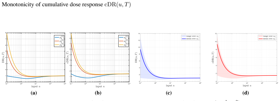
F or large u, by (28f), one has Gu(t) < 0 for every fixed t > 0 and all sufficiently large u. Therefore, ∂ucDR(u, T ) < 0. Thus, ∂ucDR(u, T ) > 0 for small u and ∂ucDR(u, T ) < 0 for large u, and hence cDR(u, T ) is not monotone. 10 -1 10 0 10 1 10 2 10 3 0 0.2 0.4 0.6 0.8 1 1.2 1.4 1.6 1.8 (a) 10 -1 10 0 10 1 10 2 10 3 0 0.5 1 1.5 2 2.5 3 (b) (c) (d) Figur...
-
[11]
Since λu(t) 0 by (29b), it follows that λu(t)gu(t) 0, 8t 2 [0, T ]
If x0 u, then by (29c), gu(t) 0 for all t 2 [0, T ]. Since λu(t) 0 by (29b), it follows that λu(t)gu(t) 0, 8t 2 [0, T ]. Hence, by Theorem 1 (i), ∂ucDR(u, T ) 0
-
[12]
Thus ˙λu(t) Gu(t) 0, 8t 2 [0, T ]
If x0 < u , then by (29e), Gu(t) 0 for all t 2 [0, T ], and by (29f), ˙λu(t) 0 for all t 2 [0, T ]. Thus ˙λu(t) Gu(t) 0, 8t 2 [0, T ]. Hence, by Theorem 1 (ii), ∂ucDR(u, T ) 0. Therefore, in either case, u 7! cDR(u, T ) is monotone nondecreasing. 18 Monotonicity of cumulative dose response cDR(u, T ) 10 -1 10 0 10 1 10 2 10 3 0 0.2 0.4 0.6 0.8 1 1.2 1.4 1...
-
[13]
By (31b), this yields Gu(t) 0 for all t 2 [0, T ]
If 0 < u x0, then xu(t) u and therefore yu(t) 1 for all t 0. By (31b), this yields Gu(t) 0 for all t 2 [0, T ]. Moreover , since ˙λu(t) 0, Theorem 1 (ii) implies ∂ucDR(u, T ) < 0
-
[14]
F or largeu, (31f) shows that, for every fixed t > 0, one has Gu(t) > 0 for all sufficiently large u. Arguing exactly as in the large- u part of System 4, this yields ∂ucDR(u, T ) > 0 for all sufficiently large u. Thus there exist u−, u+ > 0 such that ∂ucDR(u−, T ) < 0 and ∂ucDR(u+, T ) > 0, and therefore cDR(u, T ) is not monotone. 20 Monotonicity of cumula...
discussion (0)
Sign in with ORCID, Apple, or X to comment. Anyone can read and Pith papers without signing in.