PCA and t-SNE analysis in the study of QAOA entangled and non-entangled mixing operators
Pith reviewed 2026-05-24 07:56 UTC · model grok-4.3
The pith
PCA and t-SNE applied to QAOA parameters separate entangled mixing operators from non-entangled ones at depths 2L and 3L.
A machine-rendered reading of the paper's core claim, the machinery that carries it, and where it could break.
Core claim
Processing the final gate parameters of entangled and non-entangled QAOA models through PCA and t-SNE produces mappings in which entangled versions at 2L and 3L depths preserve a greater fraction of the original information, quantified by higher explained variance, while certain entangled graphs form visible clusters; the separation between the two model classes is also measured by Kullback-Leibler divergence after t-SNE optimization.
What carries the argument
Dimensionality reduction via PCA and t-SNE applied directly to the collection of optimized RZ, RX, RY parameters from entangled versus non-entangled QAOA mixing operators.
If this is right
- Entangled QAOA models at depths 2L and 3L exhibit higher explained variance in their PCA mappings than non-entangled counterparts.
- Certain entangled QAOA configurations produce visible clusters in both the PCA and t-SNE visualizations.
- Kullback-Leibler divergence after t-SNE optimization is lower for the entangled parameter sets, indicating better structure preservation.
- The numerical and visual differences between entangled and non-entangled models become more pronounced as depth increases from 1L to 3L.
Where Pith is reading between the lines
- The same visualization pipeline could be used to compare other variational quantum algorithms when entanglement is added or removed from their ansatz.
- If the separation persists across optimizers, the method offers a low-cost classical diagnostic for deciding when entanglement inside the mixer is likely to be beneficial.
- Observed clusters may correspond to distinct families of max-cut graphs or to different quality levels of the final cuts obtained.
Load-bearing premise
The final parameters reached by Stochastic Hill Climbing with Random Restarts reflect intrinsic properties of the entangled versus non-entangled QAOA models rather than artifacts of that particular optimizer or its initialization procedure.
What would settle it
Repeating the entire parameter collection and subsequent PCA/t-SNE analysis on the same max-cut instances but with a different optimizer such as gradient descent, and finding that the explained-variance gap and the clustering disappear, would falsify the claim that the observed separation is produced by the presence or absence of entanglement.
Figures


read the original abstract
In this paper, we employ PCA and t-SNE analysis to gain deeper insights into the behavior of entangled and non-entangled mixing operators within the Quantum Approximate Optimization Algorithm (QAOA) at varying depths. Our study utilizes a dataset of parameters generated for max-cut problems using the Stochastic Hill Climbing with Random Restarts optimization method in QAOA. Specifically, we examine the $RZ$, $RX$, and $RY$ parameters within QAOA models at depths of $1L$, $2L$, and $3L$, both with and without an entanglement stage inside the mixing operator. The results reveal distinct behaviors when we process the final parameters of each set of experiments with PCA and t-SNE, where in particular, entangled QAOA models with $2L$ and $3L$ present an increase in the amount of information that can be preserved in the mapping. Furthermore, certain entangled QAOA graphs exhibit clustering effects in both PCA and t-SNE. Overall, the mapping results clearly demonstrate a discernible difference between entangled and non-entangled models, quantified numerically through explained variance in PCA and Kullback-Leibler divergence (after optimization) in t-SNE, where some of these differences are also visually evident in the mapping data produced by both methods.
Editorial analysis
A structured set of objections, weighed in public.
Referee Report
Summary. The manuscript applies PCA and t-SNE to the final RZ/RX/RY parameters obtained from QAOA circuits (depths 1L, 2L, 3L) with and without an entanglement stage in the mixing operator, optimized via Stochastic Hill Climbing with Random Restarts on max-cut instances. It reports that the resulting low-dimensional mappings exhibit discernible differences, with entangled models at 2L and 3L showing higher explained variance in PCA, clustering effects, and differences in post-optimization KL divergence under t-SNE.
Significance. If the reported differences can be shown to arise from the intrinsic structure of the mixing operators rather than from optimizer-specific convergence behavior, the work would provide concrete empirical evidence that entanglement alters the geometry of optimized QAOA parameter sets, which could inform variational ansatz design. The current analysis supplies no such controls.
major comments (3)
- [experimental setup / results] The experimental dataset is never quantified: neither the number of max-cut instances nor the total number of optimized parameter vectors fed to PCA/t-SNE is stated, so the reliability of the reported explained-variance differences and clustering cannot be assessed.
- [results / discussion] No comparison of achieved approximation ratios (or final objective values) is given between the entangled and non-entangled families. Because the entangled circuits are higher-dimensional, differential convergence of SHC+RR could produce the observed parameter-structure differences even if both families reach comparable solution quality; this confound is load-bearing for the central claim.
- [t-SNE subsection] The t-SNE analysis reports KL divergence after optimization but supplies neither the perplexity values used, nor any sensitivity check to hyper-parameters or random seed, nor a statistical test that the KL differences between entangled and non-entangled cases are significant.
minor comments (3)
- [methods] The depth notation “1L, 2L, 3L” is introduced without explicit definition; clarify whether it denotes number of layers or something else.
- [figures] Figures displaying the PCA and t-SNE embeddings would benefit from consistent color or marker legends that explicitly label entangled versus non-entangled runs.
- [introduction] A brief reference to prior QAOA literature on entangling versus non-entangling mixers would help situate the empirical observations.
Simulated Author's Rebuttal
We thank the referee for their constructive comments, which highlight important aspects of clarity, controls, and statistical rigor in our analysis. We address each major comment below and commit to revisions that will strengthen the manuscript without altering its core findings.
read point-by-point responses
-
Referee: The experimental dataset is never quantified: neither the number of max-cut instances nor the total number of optimized parameter vectors fed to PCA/t-SNE is stated, so the reliability of the reported explained-variance differences and clustering cannot be assessed.
Authors: We agree that this information is missing from the manuscript. In the revised version we will explicitly report the number of max-cut instances and the total number of optimized parameter vectors supplied to PCA and t-SNE, thereby allowing readers to assess the statistical reliability of the reported differences. revision: yes
-
Referee: No comparison of achieved approximation ratios (or final objective values) is given between the entangled and non-entangled families. Because the entangled circuits are higher-dimensional, differential convergence of SHC+RR could produce the observed parameter-structure differences even if both families reach comparable solution quality; this confound is load-bearing for the central claim.
Authors: The referee correctly identifies a potential confound. We will add a direct comparison of final objective values and approximation ratios between the two families in the revised manuscript. This addition will help readers evaluate whether the observed parameter-space differences are accompanied by comparable solution quality. revision: yes
-
Referee: The t-SNE analysis reports KL divergence after optimization but supplies neither the perplexity values used, nor any sensitivity check to hyper-parameters or random seed, nor a statistical test that the KL differences between entangled and non-entangled cases are significant.
Authors: We acknowledge these omissions. The revised t-SNE subsection will report the perplexity values, include sensitivity checks across hyper-parameters and random seeds, and add a statistical test for the significance of the KL-divergence differences. revision: yes
Circularity Check
No circularity: purely empirical analysis of optimizer outputs
full rationale
The paper applies standard PCA and t-SNE dimensionality reduction to parameter vectors (RZ/RX/RY) obtained from Stochastic Hill Climbing runs on QAOA instances. Explained variance and post-optimization KL divergence are direct algorithmic outputs of these methods and do not reduce to any fitted quantity defined inside the paper. No derivation chain, first-principles prediction, or uniqueness claim is asserted; the work contains no equations that equate a result to its own inputs by construction and makes no load-bearing use of self-citations. The analysis is therefore self-contained against external benchmarks.
Axiom & Free-Parameter Ledger
axioms (1)
- domain assumption The final parameters obtained after Stochastic Hill Climbing with Random Restarts faithfully represent the optimization landscape of the QAOA model.
Reference graph
Works this paper leans on
-
[1]
A Quantum Approximate Optimization Algorithm
Farhi, E., Goldstone, J. & Gutmann, S. A quantum approximate optimization algorithm. ArXiv Preprint arXiv:1411.4028. (2014)
work page internal anchor Pith review Pith/arXiv arXiv 2014
-
[2]
Sack, S. & Serbyn, M. Quantum annealing initialization of the quantum approximate optimization algorithm. Quantum. 5 pp. 491 (2021) 12
work page 2021
-
[3]
Alam, M., Ash-Saki, A. & Ghosh, S. Accelerating quantum approximate opti- mization algorithm using machine learning. 2020 Design, Automation & Test In Europe Conference & Exhibition (DATE) . pp. 686- 689 (2020)
work page 2020
-
[4]
Shaydulin, R., Safro, I. & Larson, J. Mul- tistart methods for quantum approximate optimization. 2019 IEEE High Performance Extreme Computing Conference (HPEC) . pp. 1-8 (2019)
work page 2019
-
[5]
Koch, D., Patel, S., Wessing, L. & Alsing, P. Fundamentals in quantum algorithms: A tutorial series using Qiskit continued.ArXiv Preprint arXiv:2008.10647. (2020)
-
[6]
Galda, A., Liu, X., Lykov, D., Alexeev, Y. & Safro, I. Transferability of optimal QAOA parameters between random graphs. 2021 IEEE International Conference On Quan- tum Computing And Engineering (QCE) . pp. 171-180 (2021)
work page 2021
-
[7]
Akshay, V., Rabinovich, D., Campos, E. & Biamonte, J. Parameter concentrations in quantum approximate optimization. Physi- cal Review A. 104, L010401 (2021)
work page 2021
-
[8]
Wang, Z., Hadfield, S., Jiang, Z. & Rief- fel, E. Quantum approximate optimization algorithm for MaxCut: A fermionic view. Physical Review A. 97, 022304 (2018)
work page 2018
-
[9]
Moussa, C., Wang, H., Bäck, T. & Dunjko, V. Unsupervised strategies for identifying optimal parameters in Quantum Approximate Optimization Algorithm. EPJ Quantum Technology. 9, 11 (2022)
work page 2022
-
[10]
Vidal, R., Ma, Y., Sastry, S., Vidal, R., Ma, Y. & Sastry, S. Principal component analysis. (Springer,2016)
work page 2016
-
[11]
A Tutorial on Principal Component Analysis
Shlens, J. A tutorial on principal component analysis. ArXiv Preprint arXiv:1404.1100 . (2014)
work page internal anchor Pith review Pith/arXiv arXiv 2014
-
[12]
Maaten, L. & Hinton, G. Visualizing data using t-SNE.. Journal Of Machine Learning Research. 9 (2008)
work page 2008
-
[13]
Accelerating t-SNE using tree-based algorithms.The Journal Of Machine Learning Research
Van Der Maaten, L. Accelerating t-SNE using tree-based algorithms.The Journal Of Machine Learning Research . 15, 3221-3245 (2014)
work page 2014
-
[14]
Sarmina, B. QAOA_SHC-RR. (2023), https://github.com/BrianSarmina/ QAOA_SHC-RR
work page 2023
- [15]
-
[16]
Quantum Information Processing
Willsch, M., Willsch, D., Jin, F., De Raedt, H.&Michielsen, K.Benchmarkingthequan- tum approximate optimization algorithm. Quantum Information Processing. 19 pp. 1- 24 (2020)
work page 2020
-
[17]
Boulebnane, S. & Montanaro, A. Predicting parameters for the Quantum Approximate Optimization Algorithm for MAX-CUT from the infinite-size limit. ArXiv Preprint arXiv:2110.10685. (2021)
- [18]
-
[19]
Stęchły, M., Gao, L., Yogendran, B., Fontana, E. & Rudolph, M. Connecting the Hamiltonian structure to the QAOA energy and Fourier landscape structure. ArXiv Preprint arXiv:2305.13594. (2023)
-
[20]
Rudolph, M., Sim, S., Raza, A., Stechly, M., McClean, J., Anschuetz, E., Serrano, L. & Perdomo-Ortiz, A. ORQVIZ: Vi- sualizing High-Dimensional Landscapes in Variational Quantum Algorithms. ArXiv Preprint arXiv:2111.04695. (2021) 13 A PCA variances and graphs In this appendix, we provide additional results that complement the experiments developed to enha...
-
[21]
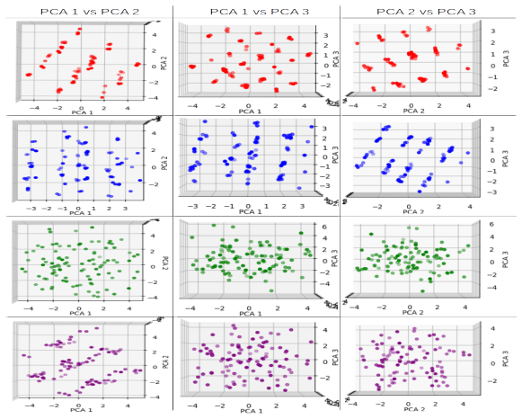
In the 3p models, both the entangled (blue) and non-entangled (red) models exhibit patterns similar to those observed in the previous 4n and 10n problems. However, there are some differences in the entangled model, particularly in the PCA 1 vs PCA 2 and PCA 1 vs PCA 3 planes, where more line patterns are observed compared to the one or two line patterns s...
-
[22]
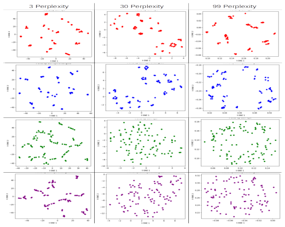
At both 3 and 30 perplexity, there is no clear pattern observed, with the distribution appearing random with no apparent clusters. At99 perplexity, there is also no distinguishable pattern observed, which is different from the elliptical behavior observed in the 10n cyclic problem but consistent with the individual PCA graphs obtained for the same problem...
discussion (0)
Sign in with ORCID, Apple, or X to comment. Anyone can read and Pith papers without signing in.