Electric field control of a quantum spin liquid in weak Mott insulators
Pith reviewed 2026-05-24 07:09 UTC · model grok-4.3
The pith
An electric field can drive a triangular lattice spin system into a chiral spin liquid by boosting ring exchange over Heisenberg terms.
A machine-rendered reading of the paper's core claim, the machinery that carries it, and where it could break.
Core claim
In the presence of an electric field the fourth-order effective ring exchange model acquires spatial anisotropy and an enhanced ring exchange term compared with the Heisenberg interaction; consequently the chiral spin liquid phase boundary shifts toward smaller t/U, so that the electric field can drive a magnetically ordered state into the chiral spin liquid.
What carries the argument
The fourth-order t/U expansion of the ring exchange Hamiltonian in an electric field, whose phase diagram is obtained by density matrix renormalization group calculations for two field directions.
If this is right
- Increasing the electric field at fixed t/U increases the relative importance of ring exchange.
- The chiral spin liquid phase boundary moves to smaller t/U for both electric field directions examined.
- A magnetically ordered state can be converted into the chiral spin liquid by raising the electric field strength.
- The same electric-field renormalization mechanism could be used to tune other quantum spin systems into spin-liquid phases.
Where Pith is reading between the lines
- Materials whose t/U ratio already lies near the zero-field boundary might enter the chiral spin liquid with experimentally accessible field strengths.
- The anisotropy induced by the field direction could produce measurable directional dependence in thermodynamic or spectroscopic signatures inside the spin-liquid regime.
- Analogous electric-field tuning might be tested on other lattices or interaction ranges where ring exchange competes with Heisenberg exchange.
Load-bearing premise
The fourth-order perturbative expansion in t/U remains accurate when the electric field is applied and correctly predicts the relative enhancement of ring exchange.
What would settle it
A direct calculation or experiment that finds the ring exchange term does not grow relative to the Heisenberg term under an applied electric field, or that the chiral spin liquid boundary does not move to smaller t/U.
Figures


read the original abstract
The triangular lattice Hubbard model at strong coupling, whose effective spin model contains both Heisenberg and ring exchange interactions, exhibits a rich phase diagram as the ratio of the hopping $t$ to onsite Coulomb repulsion $U$ is tuned. This includes a chiral spin liquid (CSL) phase. Nevertheless, this exotic phase remains challenging to realize experimentally because a given material has a fixed value of $t/U$ that can difficultly be tuned with external stimuli. One approach to address this problem is applying a DC electric field, which renormalizes the exchange interactions as electrons undergo virtual hopping processes; in addition to creating virtual doubly occupied sites, electrons must overcome electric potential energy differences. Performing a small $t/U$ expansion to fourth order, we derive the ring exchange model in the presence of an electric field and find that it not only introduces spatial anisotropy but also tends to enhance the ring exchange term compared to the dominant nearest-neighbor Heisenberg interaction. Thus, increasing the electric field serves as a way to increase the importance of the ring exchange at constant $t/U$. Through density matrix renormalization group calculations, we compute the ground state phase diagram of the ring exchange model for two different electric field directions. In both cases, we find that the electric field shifts the phase boundary of the CSL towards a smaller ratio of $t/U$. Therefore, the electric field can drive a magnetically ordered state into the CSL. This explicit demonstration opens the door to tuning other quantum spin systems into spin liquid phases via the application of an electric field.
Editorial analysis
A structured set of objections, weighed in public.
Referee Report
Summary. The paper claims that a DC electric field applied to the triangular-lattice Hubbard model at strong coupling renormalizes the effective spin Hamiltonian (derived via fourth-order t/U perturbation theory) by introducing spatial anisotropy and enhancing the ring-exchange term K relative to the Heisenberg exchange J; DMRG calculations on the resulting anisotropic ring-exchange model then show that the CSL phase boundary shifts to smaller t/U for two field directions, allowing an electric field to drive a magnetically ordered state into the CSL.
Significance. If the central result holds, the work supplies an explicit, experimentally accessible tuning knob (electric field) for entering a chiral spin liquid in a class of weak Mott insulators whose bare t/U is fixed by chemistry. The combination of a controlled perturbative derivation of the field-dependent effective model with direct DMRG phase diagrams constitutes a concrete, falsifiable prediction that could guide material searches.
major comments (2)
- [perturbative derivation] The fourth-order t/U expansion used to obtain the electric-field-dependent Heisenberg + ring-exchange model (detailed in the perturbative derivation section) is performed under the assumption that t/U remains small, yet the CSL phase reported from DMRG occurs at t/U values where this assumption is marginal; because the electric potential differences modify the energy denominators of the virtual processes, omitted sixth- and higher-order contributions can quantitatively alter the ratio K/J that controls the reported phase-boundary shift.
- [numerical results] The DMRG phase diagrams (numerical results section) for the anisotropic ring-exchange model do not report bond-dimension convergence, finite-size scaling, or boundary-condition tests; given that spin-liquid phases are known to be sensitive to these parameters, the claimed displacement of the CSL boundary cannot be assessed for robustness without such data.
minor comments (2)
- [effective model] Notation for the electric-field-induced anisotropy terms is introduced without an explicit table comparing the zero-field and finite-field coefficients; adding such a table would improve readability.
- [abstract] The abstract states that the field 'tends to enhance the ring exchange term' but does not quantify the relative change in K/J; a single sentence or inset figure summarizing the field dependence of this ratio would help readers gauge the effect size.
Simulated Author's Rebuttal
We thank the referee for their careful reading of the manuscript and for highlighting important issues regarding the perturbative expansion and the numerical robustness of the DMRG results. We address each major comment below and indicate the revisions we will make.
read point-by-point responses
-
Referee: [perturbative derivation] The fourth-order t/U expansion used to obtain the electric-field-dependent Heisenberg + ring-exchange model (detailed in the perturbative derivation section) is performed under the assumption that t/U remains small, yet the CSL phase reported from DMRG occurs at t/U values where this assumption is marginal; because the electric potential differences modify the energy denominators of the virtual processes, omitted sixth- and higher-order contributions can quantitatively alter the ratio K/J that controls the reported phase-boundary shift.
Authors: We agree that the fourth-order expansion becomes marginal at the t/U values where the CSL appears in the ring-exchange model. The derivation systematically incorporates the electric-field modifications to the energy denominators of the virtual processes at this order, which produces the reported enhancement of K relative to J. While sixth- and higher-order terms could quantitatively modify the precise location of the phase boundary, the directional effect of the field on the denominators (favoring ring-exchange processes) is expected to persist at higher orders. We will add an explicit discussion of the perturbative validity range and the possible influence of higher-order corrections in the revised manuscript. revision: partial
-
Referee: [numerical results] The DMRG phase diagrams (numerical results section) for the anisotropic ring-exchange model do not report bond-dimension convergence, finite-size scaling, or boundary-condition tests; given that spin-liquid phases are known to be sensitive to these parameters, the claimed displacement of the CSL boundary cannot be assessed for robustness without such data.
Authors: The referee is correct that the original manuscript does not present explicit convergence tests. In the revised version we will add supplementary data showing the dependence of the order parameters and entanglement entropy on bond dimension (up to at least D = 600–800), results for multiple system sizes (L = 6–12), and comparisons between open and periodic boundary conditions to confirm that the reported shift of the CSL boundary remains stable. revision: yes
Circularity Check
No circularity: standard perturbative derivation + independent DMRG
full rationale
The derivation chain consists of a conventional fourth-order t/U perturbative expansion to obtain the effective ring-exchange Hamiltonian (including E-field effects on virtual processes), followed by separate DMRG numerics on the resulting model parameters. This matches none of the enumerated circularity patterns: no self-definitional loops, no fitted inputs renamed as predictions, no load-bearing self-citations, and no ansatz or uniqueness imported from prior author work. The central claim that E-field shifts the CSL boundary is obtained from the numerical phase diagram on the independently derived Hamiltonian and does not reduce to its own inputs by construction. The expansion validity near the boundary is a correctness concern, not a circularity issue.
Axiom & Free-Parameter Ledger
axioms (1)
- domain assumption Small t/U expansion to fourth order is sufficient to capture the leading electric-field effects on ring exchange
Lean theorems connected to this paper
-
IndisputableMonolith/Cost/FunctionalEquation.leanwashburn_uniqueness_aczel unclear?
unclearRelation between the paper passage and the cited Recognition theorem.
Performing a small t/U expansion to fourth order, we derive the ring exchange model in the presence of an electric field...
-
IndisputableMonolith/Foundation/RealityFromDistinction.leanreality_from_one_distinction unclear?
unclearRelation between the paper passage and the cited Recognition theorem.
the electric field shifts the phase boundary of the CSL towards a smaller ratio of t/U
What do these tags mean?
- matches
- The paper's claim is directly supported by a theorem in the formal canon.
- supports
- The theorem supports part of the paper's argument, but the paper may add assumptions or extra steps.
- extends
- The paper goes beyond the formal theorem; the theorem is a base layer rather than the whole result.
- uses
- The paper appears to rely on the theorem as machinery.
- contradicts
- The paper's claim conflicts with a theorem or certificate in the canon.
- unclear
- Pith found a possible connection, but the passage is too broad, indirect, or ambiguous to say the theorem truly supports the claim.
Reference graph
Works this paper leans on
-
[1]
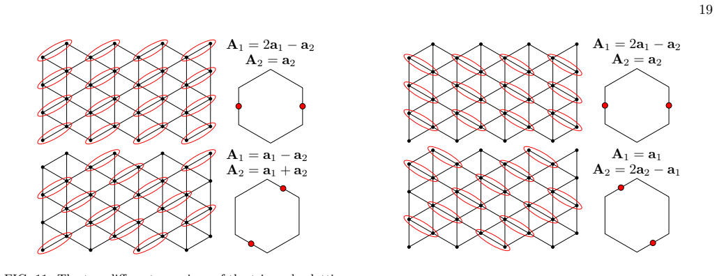
Bottom: Brillouin zone and high symmetry points of the triangular lattice
and a2 = (0 , 1) and our convention for labeling of the bonds and rings. Bottom: Brillouin zone and high symmetry points of the triangular lattice. + (Si · Sℓ)(Sj · Sk) − (Si · Sk)(Sj · Sℓ)], (19) where the detailed expressions of J(n) r (θ) are shown in Appendix B. We note that the exchange constants satisfy the typical values for the triangular lattice ...
-
[2]
Two site contributions At fourth order, there are three operator strings to consider: T −T 0T 0T +, T −T +T −T +, and T −T −T +T +. For the two site contribution, the operator string T −T 0T 0T + first creates a doubly occupied site, meaning one of the two sites is empty and the other is full. From here, there is no way to move a single electron without c...
-
[3]
Three site contributions We again consider the three operator strings: T −T 0T 0T +, T −T +T −T +, and T −T −T +T +. On three sites, again it is not possible to create two doubly occupied sites (we only have 3 electrons total, because the system is half-filled), so we have that ( T −T −T +T +)3-site = 0. We thus need to consider the other two terms. These...
-
[4]
Four site contributions The three operator strings T −T 0T 0T +, T −T +T −T +, and T −T −T +T + all contribute to the four site Hamiltonian. This time however, the T −T +T −T + term only produces “disconnected” terms, which have intermediate hoppings of the form t2 ijt2 kℓ. These disconnected terms are cancelled by further terms in T −T −T +T +. In the be...
-
[5]
(1 − α2 cos2 θ2) + 4 α2 cos2 θ1 + 2 √ 3α2 cos θ1 cos θ′ 1 + 1 (1 − α2 cos2 θ1)2 (1 − 3α2 cos2 θ′ 1) + 8 5α2 cos2 θ1 + 1 (1 − 4α2 cos2 θ1) (1 − α2 cos2 θ1)2 + 4 −α2 cos θ1 cos θ3 − √ 3α2 cos θ1 cos θ′ 3 + √ 3α2 cos θ3 cos θ′ 3 + 1 (1 − α2 cos2 θ1) (1 − α2 cos2 θ3) (1 − 3α2 cos2 θ′ 3) + 4 α2 cos2 θ1 − 2α2 cos θ1 cos θ3 + 1 (1 − α2 cos2 θ1)2 (1 − α2 cos2 θ3)...
-
[6]
(1 − α2 cos2 θ2)2 − 8 (1 − α2 cos2 θ1) (1 − α2 cos2 θ2) − 4(α2 cos2 θ1 − 2α2 cos θ1 cos θ3 + 1) (1 − α2 cos2 θ1)2 (1 − α2 cos2 θ3) − 4(α2 cos2 θ1 + 2 √ 3α2 cos θ1 cos θ′ 1 + 1) (1 − α2 cos2 θ1)2 (1 − 3α2 cos2 θ′ 1) − 8 (1 − α2 cos2 θ1) (1 − α2 cos2 θ3) + 4(α2 cos2 θ3 + 2 √ 3α2 cos θ3 cos θ′ 3 + 1) (1 − α2 cos2 θ3)2 (1 − 3α2 cos2 θ′ 3) + 4(2α2 cos θ2 cos θ...
-
[7]
(1 − α2 cos2 θ3)2 + − 4( √ 3α2 cos θ2 cos θ′ 2 + α2 cos θ2 cos θ3 + √ 3α2 cos θ′ 2 cos θ3 + 1) (1 − α2 cos2 θ2) (1 − 3α2 cos2 θ′
-
[8]
(1 − α2 cos2 θ3) − 2(α2 cos2 θ2 + 2 √ 3α2 cos θ2 cos θ′ 2 + 1) (1 − α2 cos2 θ2)2 (1 − 3α2 cos2 θ′ 2) − 2(−2α2 cos θ1 cos θ3 + α2 cos2 θ3 + 1) (1 − α2 cos2 θ1) (1 − α2 cos2 θ3)2 −2(α2 cos θ1 cos θ2 + α2 cos2 θ2 + 1) (1 − α2 cos2 θ1) (1 − α2 cos2 θ2)2 + 4 −α2 cos θ1 cos θ2 + α2 cos θ1 cos θ3 + 3α2 cos θ2 cos θ3 + 1 (1 − α2 cos2 θ1) (1 − α2 cos2 θ2) (1 − α2 ...
-
[9]
(1 − α2 cos2 θ2) # (B15) + 2t4 U3 " 2 (1 − α2 cos2 θ1) (1 − α2 cos2 θ2) − α2 cos2 θ2 + 2α2 cos θ2 cos θ3 + 1 (1 − α2 cos2 θ2)2 (1 − α2 cos2 θ3) 18 − 2 √ 3α2 cos θ′ 1 cos θ2 + α2 cos2 θ2 + 1 (1 − 3α2 cos2 θ′
-
[10]
(1 − α2 cos2 θ2)2 + 2(α2 cos θ1 cos θ2 + α2 cos θ1 cos θ3 − α2 cos θ2 cos θ3 − 1) (1 − α2 cos2 θ1) (1 − α2 cos2 θ2) (1 − α2 cos2 θ3) + 2( √ 3α2 cos θ1 cos θ′ 1 + α2 cos θ1 cos θ2 + √ 3α2 cos θ′ 1 cos θ2 + 1) (1 − α2 cos2 θ1) (1 − 3α2 cos2 θ′
-
[11]
(1 − α2 cos2 θ2) − α2 cos2 θ1 − 2α2 cos θ1 cos θ3 + 1 (1 − α2 cos2 θ1)2 (1 − α2 cos2 θ3) − α2 cos2 θ1 + 2 √ 3α2 cos θ1 cos θ′ 1 + 1 (1 − α2 cos2 θ1)2 (1 − 3α2 cos2 θ′ 1) # J(1) 3 (θ) = 4t4 U3 " 2 1 + α2 cos2 θ1 (1 − α2 cos2 θ1)3 − 5α2 cos2 θ1 + 1 (1 − 4α2 cos2 θ1) (1 − α2 cos2 θ1)2 # (B16) J(1) r (θ) = 8t4 U3 " 2 (1 − α2 cos2 θ1) (1 − α2 cos2 θ2) + α2 cos...
-
[12]
(1 − α2 cos2 θ2) +2 √ 3α2 cos θ′ 1 cos θ2 + α2 cos2 θ2 + 1 (1 − 3α2 cos2 θ′
-
[13]
(1 − α2 cos2 θ2)2 + α2 cos2 θ1 + 2 √ 3α2 cos θ1 cos θ′ 1 + 1 (1 − α2 cos2 θ1)2 (1 − 3α2 cos2 θ′ 1) # . We note that, in order to obtain the coupling constants along different bonds, we may use J(2) 1 (θ) = J(1) 1 (θ − π/3), and J(3) 1 (θ) = J(1) 1 (θ − 2π/3). The same relations hold for the second and third nearest neighbors, as well as the ring exchange....
-
[14]
Perform this initialization run with 5 sweeps and a chiral symmetry breaking term of Jχ = 10−5
First, initialize the system with an up/down prod- uct state, and maximum bond dimension of b = 20. Perform this initialization run with 5 sweeps and a chiral symmetry breaking term of Jχ = 10−5
-
[15]
Now, set Jχ = 0. Take the output of the first step as the initial state for a run with the density matrix mixer on to escape local minima, with a maximum of 40 sweeps and bond dimension of b = 1600
-
[16]
This is also done with bond dimension b = 1600
Take the output of the second step as the initial state for a run with the density matrix mixer off because we assume that we are in the global mini- mum basin, and run until the energy converges to ∆E = 10−8. This is also done with bond dimension b = 1600. Sometimes, the simulation converges in energy, but does not converge to the true ground state. This...
-
[17]
Dimer Coverings of the Triangular lattice As mentioned in the main text, there are 6 simple dimer coverings of the triangular lattice. This is not an 19 A1=2a1a2 A2=a2 A1=a1a2 A2=a1+a2 A1=a1 A2=2a2a1 A1=a1a2 A2=a1+a2 A1=2a1a2 A2=a2 A1=a1 A2=2a2a1 164 FIG. 11. The two different coverings of the triangular lattice by dimers along the a1 bond. The two transl...
-
[18]
Valence bond solid 1 There are 6 possible simple dimer coverings of the tri- angular lattice. To identify the VBS 1 state with particu- lar dimer coverings, we compute the three different dimer A1=2a1a2 A2=a2 A1=a1a2 A2=a1+a2 A1=a1 A2=2a2a1 A1=a1a2 A2=a1+a2 A1=2a1a2 A2=a2 A1=a1 A2=2a2a1 163 FIG. 13. The two different coverings of the triangular lattice by...
-
[19]
The peaks are at the M ′′ points
Valence bond solid 2 For VBS2, the dimer structure factor with the largest peak height is the one along the a2. The peaks are at the M ′′ points. Identifying this with the configurations in Fig. 12, we find the wave function in Eq. (26)
-
[20]
The dimer correlations are long-ranged, as can be seen in Figs
Valence bond solid 3 The third valence bond solid has strong dimer corre- lations, but not at high symmetry points. The dimer correlations are long-ranged, as can be seen in Figs. 19-
-
[21]
This suggests that this phase is a valence bond solid whose unit cell is larger than the size of our finite sized simulation. Appendix E: DMRG Data
-
[22]
(E1) The spin structure factor is primarily used to identify magnetically ordered phases
Spin Structure Factor The spin structure factor is defined by 20 S(k) = X ij eik·(Ri−Rj)(⟨Si · Sj⟩ − ⟨Si⟩ · ⟨Sj⟩). (E1) The spin structure factor is primarily used to identify magnetically ordered phases. The peaks of the momen- tum space spin structure factor should be at high sym- metry points in the Brillouin zone, and also be sharp, indicating long ra...
-
[23]
Dimer Structure Factors We define the dimer operator Dn i (k) = Si ·Si+an. This structure factor probes the formation of singlets between nearest-neighbor spins in the lattice along the an direc- tion. Then, we define the dimer structure factor by Dn(k) = X ij eik·(Ri−Rj)(⟨Dn i Dn j ⟩ − ⟨Dn i ⟩⟨Dn j ⟩). (E2)
-
[24]
Entanglement Spectrum As mentioned in the main text, the entanglement spec- trum is obtained by considering the mixed transfer ma- trix T T α1α2α3α4, which is constructed by translating the wavefunction |ψ⟩ by one lattice spacing along the cir- cumferential direction, and then contracting its physical indices with those of the original (untranslated) wave...
- [25]
- [26]
-
[27]
J. Knolle and R. Moessner, Annu. Rev. Condens. Matter Phys. 10, 451 (2019)
work page 2019
-
[28]
Y. Zhou, K. Kanoda, and T.-K. Ng, Rev. Mod. Phys. 89, 025003 (2017)
work page 2017
-
[29]
C. Broholm, R. J. Cava, S. A. Kivelson, D. G. Nocera, M. R. Norman, and T. Senthil, Science 367, eaay0668 (2020)
work page 2020
- [30]
- [31]
- [32]
-
[33]
Anderson, Materials Research Bulletin 8, 153 (1973)
P. Anderson, Materials Research Bulletin 8, 153 (1973)
work page 1973
-
[34]
J. S. Gordon, A. Catuneanu, E. S. Sørensen, and H.-Y. Kee, Nat Commun 10, 2470 (2019)
work page 2019
-
[35]
E. S. Sørensen, A. Catuneanu, J. S. Gordon, and H.-Y. Kee, Phys. Rev. X 11, 011013 (2021)
work page 2021
-
[36]
H.-S. Kim, Y. B. Kim, and H.-Y. Kee, Phys. Rev. B 94, 245127 (2016)
work page 2016
- [37]
-
[38]
S.-H. Baek, S.-H. Do, K.-Y. Choi, Y. Kwon, A. Wolter, S. Nishimoto, J. Van Den Brink, and B. B¨ uchner, Phys. Rev. Lett. 119, 037201 (2017)
work page 2017
-
[39]
Y. Kasahara, T. Ohnishi, Y. Mizukami, O. Tanaka, S. Ma, K. Sugii, N. Kurita, H. Tanaka, J. Nasu, Y. Mo- tome, T. Shibauchi, and Y. Matsuda, Nature 559, 227 (2018)
work page 2018
-
[40]
H.-Y. Lee, R. Kaneko, L. E. Chern, T. Okubo, Y. Yamaji, N. Kawashima, and Y. B. Kim, Nat Commun 11, 1639 (2020)
work page 2020
-
[41]
L. E. Chern, R. Kaneko, H.-Y. Lee, and Y. B. Kim, Phys. Rev. Research 2, 013014 (2020)
work page 2020
-
[42]
H. Li, Y. B. Kim, and H.-Y. Kee, Phys. Rev. B 105, 245142 (2022)
work page 2022
- [43]
-
[44]
R. Sano, Y. Kato, and Y. Motome, Phys. Rev. B 97, 014408 (2018)
work page 2018
- [45]
-
[46]
S. Sur, A. Udupa, and D. Sen, Phys. Rev. B 105, 054423 (2022)
work page 2022
-
[47]
A. H. MacDonald, S. M. Girvin, and D. Yoshioka, Phys. Rev. B 37, 9753 (1988)
work page 1988
- [48]
-
[49]
J.-Y. P. Delannoy, M. J. P. Gingras, P. C. W. Holdsworth, and A.-M. S. Tremblay, Phys. Rev. B 72, 115114 (2005)
work page 2005
-
[50]
T. Cookmeyer, J. Motruk, and J. E. Moore, Phys. Rev. Lett. 127, 087201 (2021)
work page 2021
- [51]
- [52]
-
[53]
A. Bose, A. Haldar, E. S. Sørensen, and A. Paramekanti, Phys. Rev. B 107, L020411 (2023)
work page 2023
-
[54]
T. Shirakawa, T. Tohyama, J. Kokalj, S. Sota, and S. Yunoki, Phys. Rev. B 96, 205130 (2017)
work page 2017
- [55]
-
[56]
S.-S. Gong, W. Zhu, and D. N. Sheng, Sci Rep 4, 6317 (2014)
work page 2014
- [57]
- [58]
-
[59]
T. Tang, B. Moritz, and T. P. Devereaux, Phys. Rev. B 106, 064428 (2022)
work page 2022
-
[60]
L. F. Tocchio, A. Montorsi, and F. Becca, Phys. Rev. Research 3, 043082 (2021)
work page 2021
-
[61]
B.-B. Chen, Z. Chen, S.-S. Gong, D. N. Sheng, W. Li, and A. Weichselbaum, Phys. Rev. B 106, 094420 (2022)
work page 2022
- [62]
-
[63]
Y. Zhou, D. Sheng, and E.-A. Kim, Phys. Rev. Lett. 128, 157602 (2022)
work page 2022
-
[64]
J. Willsher, H.-K. Jin, and J. Knolle, Phys. Rev. B 107, 064425 (2023)
work page 2023
- [65]
- [66]
- [67]
-
[68]
P. Sahebsara and D. S´ en´ echal, Phys. Rev. Lett. 100, 136402 (2008)
work page 2008
- [69]
- [70]
-
[71]
S.-S. Gong, W. Zheng, M. Lee, Y.-M. Lu, and D. N. Sheng, Phys. Rev. B 100, 241111 (2019)
work page 2019
-
[72]
Y. Huang, D. N. Sheng, and J.-X. Zhu, (2023), 10.48550/ARXIV.2306.03056, publisher: arXiv Version Number: 1
- [73]
- [74]
-
[75]
S. C. Furuya, K. Takasan, and M. Sato, Phys. Rev. Re- search 3, 033066 (2021)
work page 2021
-
[76]
S. C. Furuya and M. Sato, (2021), 10.48550/ARXIV.2110.06503, publisher: arXiv Ver- sion Number: 2
- [77]
- [78]
- [79]
- [80]
discussion (0)
Sign in with ORCID, Apple, or X to comment. Anyone can read and Pith papers without signing in.