Convolutional Maximum Mean Discrepancy for Inference in Noisy Data
Pith reviewed 2026-05-10 15:05 UTC · model grok-4.3
The pith
Convolutional maximum mean discrepancy enables consistent inference from samples corrupted by known measurement noise.
A machine-rendered reading of the paper's core claim, the machinery that carries it, and where it could break.
Core claim
The central claim is that convMMD, defined as the MMD between the noise-convolved versions of the two distributions, is a valid metric under standard kernel conditions and admits finite-sample concentration inequalities independent of the noise level. This quantity is equivalent to a kernel-smoothed comparison of the clean distributions. The paper uses this equivalence to construct an estimator for the discrepancy that remains consistent and asymptotically normal when observations are heteroscedastically noisy, with an SGD implementation that scales to large samples.
What carries the argument
convMMD, the maximum mean discrepancy computed after convolving each of the two distributions with the known noise distribution.
If this is right
- Finite-sample deviation bounds for the empirical convMMD hold regardless of noise strength or heteroscedasticity.
- Testing whether two noisy samples come from the same distribution is equivalent to a kernel-smoothed test on the clean distributions.
- The convMMD estimator is consistent and asymptotically normal, supporting standard confidence intervals and p-values.
- Stochastic gradient descent yields a practical algorithm for computing or optimizing the statistic on large datasets.
Where Pith is reading between the lines
- The framework could be extended to cases where the noise distribution is estimated rather than known exactly, provided separate error bounds control the plug-in uncertainty.
- convMMD offers a kernel-based route to inference without needing to recover the full noise-free density via classical deconvolution.
- Similar convolution adjustments might apply to other kernel embeddings or discrepancy measures when data arrive with additive noise.
Load-bearing premise
The measurement noise distribution is known exactly and the base kernel satisfies the standard conditions that make MMD a metric.
What would settle it
In repeated simulations that draw clean samples from two identical distributions, add noise from the known distribution, and compute empirical convMMD, the statistic fails to converge to zero at the rate given by the finite-sample bounds.
Figures


read the original abstract
Modern data analyses frequently encounter settings where samples of variables are contaminated by measurement error. Ignoring measurement noise can substantially degrade statistical inference, while existing correction techniques are often computationally costly and inefficient. Recent advances in kernel methods, particularly those based on Maximum Mean Discrepancy (MMD), have enabled flexible, distribution-free inference, yet typically assume precise data and overlook contamination by measurement error. In this work, we introduce a novel framework for inference with samples corrupted by potentially heteroscedastic noise from a known distribution. Central to our approach is the convolutional MMD (convMMD), which compares distributions after noise convolution and retains metric validity under standard kernel conditions. We establish finite-sample deviation bounds that are unaffected by measurement error and prove an equivalence between testing under noise and kernel smoothing. Leveraging these insights, we introduce a convMMD-based estimator for inference with noisy, heteroscedastic observations. We establish its consistency and asymptotic normality, and provide an efficient implementation using stochastic gradient descent. We demonstrate the practical effectiveness of our approach through simulations and applications in astronomy and social sciences.
Editorial analysis
A structured set of objections, weighed in public.
Referee Report
Summary. The paper introduces a convolutional Maximum Mean Discrepancy (convMMD) framework for nonparametric inference on distributions when samples are corrupted by known, potentially heteroscedastic measurement noise. It claims that convMMD compares convolved distributions while preserving metric properties under standard kernel conditions, derives finite-sample deviation bounds independent of the noise, establishes an equivalence between noisy testing and kernel smoothing, and develops a consistent, asymptotically normal convMMD-based estimator that can be optimized efficiently via stochastic gradient descent. The approach is illustrated with simulations and applications in astronomy and social sciences.
Significance. If the central theoretical claims hold, particularly the noise-independent finite-sample bounds and the consistency/asymptotic normality of the estimator, the work would offer a practical and theoretically grounded extension of MMD-based methods to noisy data settings common in observational sciences. The equivalence to kernel smoothing and the SGD implementation could enable scalable inference without the computational overhead of existing correction techniques.
major comments (2)
- [Theoretical results on deviation bounds] The abstract asserts finite-sample deviation bounds for convMMD that are unaffected by measurement error. The main theorem establishing these bounds (presumably in the theoretical results section) must be checked to confirm that the known noise distribution is used to cancel all additive variance terms exactly in the concentration inequality, with no residual dependence on noise variance or per-sample heteroscedasticity parameters remaining in the final rate or constants. Without this explicit cancellation, the 'unaffected' guarantee would not hold under stronger contamination.
- [Section on equivalence to kernel smoothing] The claimed equivalence between testing under noise and kernel smoothing is central to the framework but requires a precise statement of the conditions under which the convMMD statistic reduces to a smoothed kernel test. If this equivalence is used to justify the estimator's properties, the proof should clarify whether it holds only for specific kernels or more generally.
minor comments (2)
- [Introduction or preliminaries] The abstract mentions 'standard kernel conditions' for metric validity; these should be stated explicitly (e.g., characteristic kernels) in the main text for clarity.
- [Implementation section] Details on the SGD implementation, including convergence criteria and hyperparameter choices, would benefit from a dedicated algorithmic description or pseudocode.
Simulated Author's Rebuttal
We thank the referee for their thorough review and constructive comments on our manuscript. We address each major comment below, confirming the validity of our theoretical claims while agreeing to add clarifications for precision. We believe these revisions will strengthen the presentation without altering the core results.
read point-by-point responses
-
Referee: [Theoretical results on deviation bounds] The abstract asserts finite-sample deviation bounds for convMMD that are unaffected by measurement error. The main theorem establishing these bounds (presumably in the theoretical results section) must be checked to confirm that the known noise distribution is used to cancel all additive variance terms exactly in the concentration inequality, with no residual dependence on noise variance or per-sample heteroscedasticity parameters remaining in the final rate or constants. Without this explicit cancellation, the 'unaffected' guarantee would not hold under stronger contamination.
Authors: We confirm that the main theorem (Theorem 3.1) establishes the finite-sample deviation bounds precisely by incorporating the known noise distribution into the definition of convMMD. This allows the additive variance terms from the measurement error to cancel exactly in the concentration inequality, as the statistic is defined on the convolved distributions. The resulting bounds depend only on the kernel and the original (unobserved) distributions, with no residual dependence on noise variance or heteroscedasticity parameters. We will add an explicit remark following the theorem statement to highlight this cancellation mechanism and its implications for stronger contamination settings. revision: yes
-
Referee: [Section on equivalence to kernel smoothing] The claimed equivalence between testing under noise and kernel smoothing is central to the framework but requires a precise statement of the conditions under which the convMMD statistic reduces to a smoothed kernel test. If this equivalence is used to justify the estimator's properties, the proof should clarify whether it holds only for specific kernels or more generally.
Authors: We agree that precision is needed here. The equivalence is stated in Proposition 4.1 and holds generally for any characteristic kernel (i.e., any positive definite kernel that metrizes the space of probability measures), without restriction to specific families such as Gaussian or Matérn kernels. The proof uses the reproducing property of the RKHS together with the convolution operation and does not rely on kernel-specific features beyond the standard characteristic assumption. In the revision, we will restate the proposition with the exact conditions listed explicitly and add a sentence clarifying its generality. revision: yes
Circularity Check
No circularity in derivation chain
full rationale
The paper defines convMMD directly via convolution of the base kernel with the known noise distribution and proves it inherits metric properties under standard kernel conditions. Finite-sample deviation bounds are stated to be unaffected by measurement error, with consistency and asymptotic normality following from extensions of existing MMD theory rather than any reduction to fitted inputs or self-referential definitions. No steps match the enumerated circularity patterns: no self-definitional quantities, no predictions that are statistically forced by construction, no load-bearing self-citations for uniqueness or ansatz, and no renaming of known results. The framework is self-contained against external kernel-method benchmarks.
Axiom & Free-Parameter Ledger
axioms (2)
- domain assumption The measurement noise distribution is known exactly
- domain assumption The base kernel satisfies standard conditions that make MMD a metric
invented entities (1)
-
convMMD
no independent evidence
Reference graph
Works this paper leans on
-
[1]
(Generalization Bound) With probability 1−γ, we have convMMD p, qbθN , m ≤inf θ∈Θ convMMD (p, qθ, m) + 4 r 2K N ! (2 + p log(1/γ)),
-
[2]
That is lim N→∞ bθN =θ ⋆ almost surely
(Consistency) The empirical convMMD estimator bθN converges almost surely toθ ⋆ if it is fitted on noisy data and samples of sizeNfromq θ ∗m. That is lim N→∞ bθN =θ ⋆ almost surely. ProofThe bound and consistency result follows directly from Theorem 1 and Proposition 1 in Briolet al.(2019). They derived the bound for the case when we have access to sample...
work page 2019
-
[7]
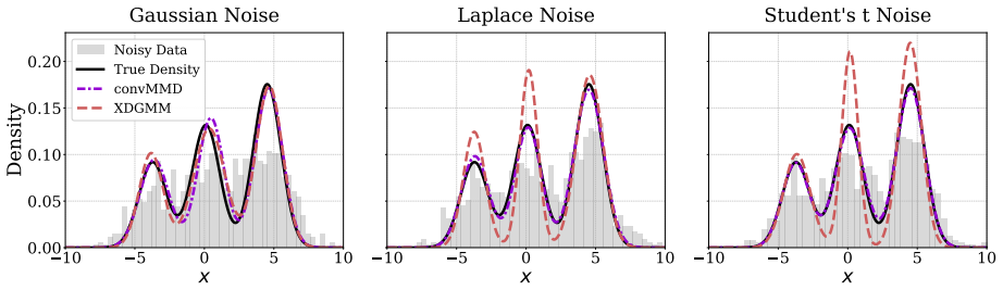
Student’s t (Heteroscedastic):U Xi, UYi ∼r(·|ϕ) =ϕ·t(3), whereϕ∼g(·|ψ) =√ 3U(1,1.5). For XDGMM, we provide the true error standard deviation in case of homoscedastic noise processes as a parameter to the method. In the case of heteroscedastic noise processes, we provide point-wise error standard deviations that are derived from the conditional distribu- t...
-
[8]
True Covariate (X): The true covariate distribution is a two-component Gaussian mixture: X∼0.3N 2.5,1 2 + 0.7N 3,1 2
-
[9]
Thus, given the above data generating process, we haveθ reg = (α, β, σ reg)
True Response (Y) : The true response is generated via a linear relationship with additive Gaussian noise: Y= 1.5 +X+ε, ε∼ N 0,1 2 . Thus, given the above data generating process, we haveθ reg = (α, β, σ reg). The observed noisy samples eXand eYare generated by adding measurement noise to clean data. We used several noise configurations to demonstrate the...
-
[10]
Gaussian (Homoscedastic):U Xi, UYi ∼r(·|ϕ) =N(0, ϕ 2), whereϕ= 1.258
-
[11]
Uniform (Homoscedastic):U Xi, UYi ∼r(·|ϕ) =U(−ϕ, ϕ), whereϕ= 2
-
[12]
Gaussian (Heteroscedastic):U Xi, UYi ∼r(·|ϕ) =N(0, ϕ 2), whereϕ∼g(·|ψ) = U(1,1.5)
-
[13]
Laplace (Heteroscedastic):U Xi, UYi ∼r(·|ϕ) = Laplace(0, ϕ), whereϕ∼g(·|ψ) =√ 2U(1,1.5)
-
[14]
Student’s t (Heteroscedastic):U Xi, UYi ∼r(·|ϕ) =ϕ·t(3), whereϕ∼g(·|ψ) =√ 3U(1,1.5). Supplementary Materials S.26 0.5 1.0 1.5 2.0 2.5 Estimated Intercept ( ) 0.00 0.25 0.50 0.75 1.00 1.25 1.50Density (a) Distribution of for convMMD CLT Density (N(1.52, 0.29)) True Value (1.5) Mean Est (1.5) 0.6 0.7 0.8 0.9 1.0 1.1 1.2 1.3 1.4 Estimated Residual Std ( ) 0 ...
work page 1994
-
[15]
Variable Income:U Income ∼r(· |ϕ) =N(0, ϕ 2), whereϕ= 0.8. Effective variance = 0.64
-
[16]
This formulation ensures zero-mean noise with an effective variance of 0.75
Variable Age:U Age ∼r(· |ϕ) = 0.5·(Poisson(ϕ)−ϕ), whereϕ= 3. This formulation ensures zero-mean noise with an effective variance of 0.75. 2Publicly available athttps://github.com/afarahi/American-Housing-Survey-Study- Supplementary Materials S.29 We modeled the latent distribution of the true covariatesXAge andX Income using independent GMM models withK= ...
discussion (0)
Sign in with ORCID, Apple, or X to comment. Anyone can read and Pith papers without signing in.