Horseshoe Predictive Inference
Pith reviewed 2026-05-10 06:40 UTC · model grok-4.3
The pith
The Horseshoe prior delivers asymptotically minimax optimal predictive Bayes estimators in sparse Gaussian sequence models.
A machine-rendered reading of the paper's core claim, the machinery that carries it, and where it could break.
Core claim
The predictive Bayes estimator under the Horseshoe prior is exactly asymptotically minimax optimal when sparsity is known. Through Horseshoe spectroscopy, the phase-transition in the local shrinkage scale is passed to the predictive mechanism. When sparsity is unknown, the hierarchical Horseshoe performs adaptive switching and attains an upper bound on predictive risk over a restricted parameter class that improves on the minimax rate for the full class, provided a theta-min condition holds.
What carries the argument
Horseshoe spectroscopy, a Gaussian-mixture representation of the posterior predictive density that transfers the phase transition from the shrinkage scale to the predictive inference step.
If this is right
- The predictive Horseshoe estimator matches the minimax rate for known sparsity levels in sparse Gaussian sequences.
- Hierarchical Horseshoe priors allow automatic adaptation to unknown sparsity without manual tuning.
- Predictive risk bounds improve under theta-min conditions for signals in restricted classes.
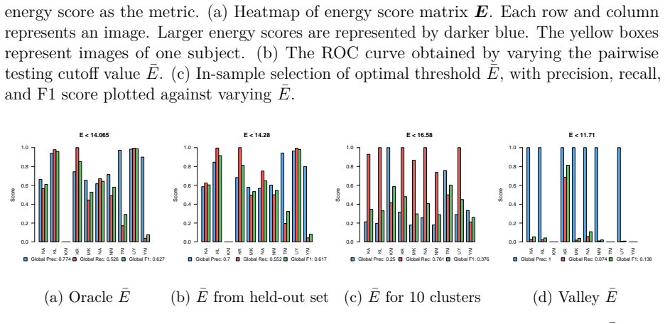
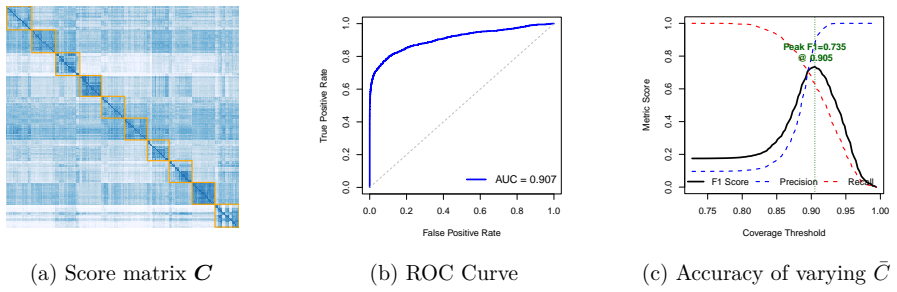
- The approach applies directly to modeling images and time series as sparse Gaussian sequences for tasks like facial recognition.
Where Pith is reading between the lines
- If the spectroscopy mechanism generalizes, other continuous shrinkage priors might exhibit similar phase-transition inheritance in prediction.
- This could lead to better uncertainty quantification in sparse predictive settings compared to discrete mixture priors.
- Testing on additional domains like genomics or finance could validate the practical gains from adaptive switching.
Load-bearing premise
The theta-min condition on the signals is required to obtain the sharper upper bound on predictive risk over the restricted parameter class when sparsity is unknown.
What would settle it
If the predictive risk under the hierarchical Horseshoe exceeds the claimed upper bound in simulations satisfying the theta-min condition, or if the posterior predictive density fails to exhibit the phase transition in local shrinkage for known sparsity, the central claims would not hold.
Figures


read the original abstract
Predictive inference in the sparse Gaussian sequence model has received considerably less attention than its non-sparse, finite-sample counterpart. Existing work has largely been confined to discrete mixture priors. In this paper, we study predictive inference under a widely used continuous mixture prior, the Horseshoe. We provide new theoretical results establishing exact asymptotic minimax optimality of the predictive Bayes estimator when the sparsity level is known. Furthermore, through a Gaussian-mixture representation of the posterior predictive density (which we term Horseshoe spectroscopy), the phase-transition in the local shrinkage scale is inherited by the predictive mechanism, producing behavior similar to that of previous thresholding/switching estimators. When sparsity is unknown, we adopt a fully Bayesian approach using a hierarchical Horseshoe prior and show that it performs adaptive, as opposed to manual, switching. Under a theta-min condition, the resulting predictive risk admits an upper bound over a restricted parameter class that is sharper than the minimax rate over the full class. We demonstrate the practical value of predictive Horseshoe shrinkage on data such as images and time series that can be naturally modeled as sparse Gaussian sequences. We illustrate this approach on facial recognition across varying facial expressions and study region-wise atypical brain lateralization in autism spectrum disorder.
Editorial analysis
A structured set of objections, weighed in public.
Referee Report
Summary. The manuscript claims to establish exact asymptotic minimax optimality of the predictive Bayes estimator under the Horseshoe prior in the sparse Gaussian sequence model when sparsity is known. It introduces 'Horseshoe spectroscopy' as a Gaussian-mixture representation of the posterior predictive density to demonstrate inheritance of the local shrinkage phase-transition to prediction. For unknown sparsity, the hierarchical Horseshoe prior is shown to perform adaptive switching, and under a theta-min condition, the predictive risk admits a sharper upper bound over a restricted parameter class than the minimax rate over the full class. Practical value is demonstrated on image and time series data for applications like facial recognition and brain lateralization analysis in autism spectrum disorder.
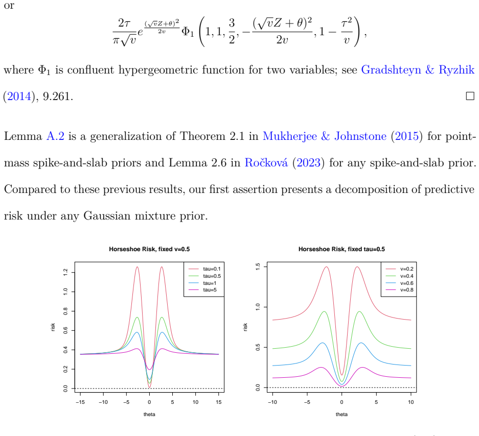
Significance. Should the theoretical results be verified, this paper contributes meaningfully to the literature on Bayesian predictive inference in sparse high-dimensional settings by providing rigorous optimality guarantees for a popular continuous shrinkage prior. The Horseshoe spectroscopy offers a fresh perspective on how shrinkage mechanisms translate to predictive distributions, potentially generalizable to other priors. The adaptive results under the hierarchical prior, albeit restricted, advance understanding of fully Bayesian approaches to unknown sparsity. The real-data examples underscore the method's relevance to statistical applications in imaging and neuroscience.
major comments (1)
- [Abstract and unknown sparsity section] Abstract and section on unknown sparsity: The upper bound on predictive risk that is sharper than the minimax rate over the full class is derived under the theta-min condition on the signals. This condition is load-bearing for the adaptivity claim as it excludes arbitrarily small signals; without it, the risk may not improve. The manuscript should explicitly state whether this restriction is necessary or if extensions to the full class are possible.
minor comments (3)
- [Introduction] The term 'Horseshoe spectroscopy' is coined for the Gaussian-mixture representation of the posterior predictive density; a formal definition and motivation should be provided at the first mention to aid reader comprehension.
- [Applications] The modeling of images and time series as sparse Gaussian sequences in the applications could benefit from more explicit description of the data transformation steps and how the sequence model is fitted.
- [Introduction] Additional references to prior work on predictive inference using discrete mixture priors in sparse models would better position the continuous Horseshoe approach.
Simulated Author's Rebuttal
We thank the referee for their thoughtful review and positive assessment of the manuscript. We address the single major comment below and will revise the paper accordingly to improve clarity.
read point-by-point responses
-
Referee: [Abstract and unknown sparsity section] Abstract and section on unknown sparsity: The upper bound on predictive risk that is sharper than the minimax rate over the full class is derived under the theta-min condition on the signals. This condition is load-bearing for the adaptivity claim as it excludes arbitrarily small signals; without it, the risk may not improve. The manuscript should explicitly state whether this restriction is necessary or if extensions to the full class are possible.
Authors: We agree that the theta-min condition plays a central role in deriving the sharper upper bound, as it ensures signals are bounded away from zero and thereby permits the hierarchical Horseshoe to achieve adaptive switching without interference from arbitrarily small nonzero components. Without this separation, the predictive risk may revert to the minimax rate over the full class. In the revised manuscript we will explicitly state that the restriction is necessary for the improved bound and that extending the result to the unrestricted class (without a theta-min condition) is an open question left for future work. This clarification will be added to both the abstract and the unknown-sparsity section. revision: yes
Circularity Check
No circularity: standard minimax and Bayesian derivations on Horseshoe prior
full rationale
The paper derives exact asymptotic minimax optimality for the predictive Bayes estimator under known sparsity using standard theoretical techniques for continuous mixture priors in the Gaussian sequence model. The Horseshoe spectroscopy representation is introduced as a Gaussian-mixture form of the posterior predictive density to transfer local shrinkage phase transitions, but this is an analytical tool rather than a self-definitional reduction or fitted input renamed as prediction. The adaptive result for unknown sparsity employs a hierarchical Horseshoe prior with an explicit theta-min condition on signals to obtain a sharper upper bound on a restricted class; this is a stated assumption, not a circular equivalence or self-citation load-bearing step. No equations or claims reduce by construction to the paper's own inputs, prior self-citations, or renamings of known empirical patterns. The derivation chain remains self-contained against external minimax benchmarks.
Axiom & Free-Parameter Ledger
axioms (2)
- domain assumption Observations follow the sparse Gaussian sequence model y_i = theta_i + epsilon_i with epsilon_i ~ N(0,1)
- domain assumption The Horseshoe prior induces the desired shrinkage and phase-transition behavior
invented entities (1)
-
Horseshoe spectroscopy
no independent evidence
Reference graph
Works this paper leans on
-
[1]
Assume that the prior ofθis a scale-mixture of Gaussians,θ|λ∼N(0,λ2), where the prior ofλisν(λ), then ρ(θ,ˆp) =θ2 2r−EθlogN GM θ,v(Z) +E θlogN GM θ,1(Z),(A.1) where NGM θ,v(Z) = ∫ ∞ 0 √ v λ2 +v exp [ λ2 λ2 +v (√vZ+θ)2 2v ] ν(λ) dλ
-
[2]
Specifically, ifθfollows Horseshoe prior with a fixedτ >0, then ρ(θ,ˆp) =θ2 2r−EθlogN HS θ,v(Z) +E θlogN HS θ,1(Z),(A.2) whereN HS θ,v(Z)takes any of the following equivalent forms: NHS θ,v(Z) = τ π√v ∫ 1 0 u−1/2 1 τ2/v+ (1−τ2/v)u exp [ (√vZ+θ)2 2v u ] du(A.3) = τ π√ve (√vZ+θ)2 2v ∫ 1 0 (1−u)−1/2 1 1−(1−τ2/v)u exp [ −(√vZ+θ)2 2v u ] du (A.4) = 2τ π√ve (√v...
work page 2014
-
[3]
Forτ∈(0, 1), we may boundD(Yi)from above and Nv(Yi, ˜Yi)from below
Recall Lemma C.1 that ˜g(Yi, ˜Yi,θi,v) = ˜Yiθi r −θ2 i 2r−logNv(Yi, ˜Yi) + logD(Yi). Forτ∈(0, 1), we may boundD(Yi)from above and Nv(Yi, ˜Yi)from below. Using the representation (C.1), we haveτ2 + (1−τ2)u≥τ2 forτ∈(0,1), and hence logD(Yi)≤log ( τ π·eY 2 i /2 τ2 ∫ 1 0 u−1/2du ) = Y 2 i 2 + log 1 τ+ log 2 π. Meanwhile, note thatτ2/v+ (1−τ2/v)u≤1/vforτ∈(0,1)...
work page 2023
-
[4]
Boxplots display the distribution of these scores for the ASD group (red) and control group (blue)
Cerebellum_10 0.0 0.5 1.0 0.0 0.5 1.0 0.0 0.5 1.0 Rank−based Predictive Score Group ASD Control Figure 17: Distribution of rank-based predictive scores across 54 brain regions. Boxplots display the distribution of these scores for the ASD group (red) and control group (blue). Region labels are color-coded based on significant group differences in Wilcoxon...
-
[5]
Boxplots display the distribution of these scores for the ASD group (red) and control group (blue)
Cerebellum_10 0.0 0.5 1.0 0.0 0.5 1.0 0.0 0.5 1.0 Entrywise Coverage Rate (C) Group ASD Control Figure 19: Distribution of coverage rates across 54 brain regions. Boxplots display the distribution of these scores for the ASD group (red) and control group (blue). Region labels are color-coded based on significant group differences in Wilcoxon rank-sum test...
discussion (0)
Sign in with ORCID, Apple, or X to comment. Anyone can read and Pith papers without signing in.