A Linear Method for Shape Reconstruction based on the Generalized Multiple Measurement Vectors Model
Pith reviewed 2026-05-25 15:43 UTC · model grok-4.3
The pith
A GMMV-based linear method reconstructs shapes from electromagnetic scattering data more sharply than the linear sampling method.
A machine-rendered reading of the paper's core claim, the machinery that carries it, and where it could break.
Core claim
The GMMV-based linear method, which solves contrast sources iteratively under a joint sparsity constraint with cross-validation termination, produces shape reconstructions from TM experimental data that focus better than those from the linear sampling method.
What carries the argument
Generalized multiple measurement vectors model applied to contrast sources, with joint sparsity as the regularizer and cross-validation for automatic iteration stopping.
Load-bearing premise
The joint sparsity constraint on contrast sources combined with cross-validation termination produces stable and accurate shape estimates without explicit knowledge of the noise level or additional regularization tuning.
What would settle it
A controlled comparison on the same TM experimental data set, with known ground-truth shapes, that measures whether the reported focusing advantage disappears when the noise level is supplied to both methods or when the sparsity level is deliberately mismatched.
Figures


read the original abstract
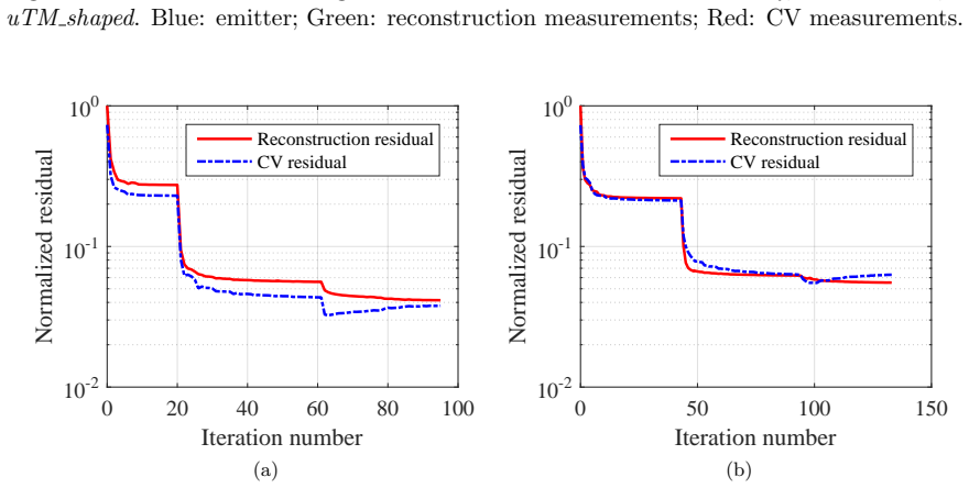
In this paper, a novel linear method for shape reconstruction is proposed based on the generalized multiple measurement vectors (GMMV) model. Finite difference frequency domain (FDFD) is applied to discretized Maxwell's equations, and the contrast sources are solved iteratively by exploiting the joint sparsity as a regularized constraint. Cross validation (CV) technique is used to terminate the iterations, such that the required estimation of the noise level is circumvented. The validity is demonstrated with an excitation of transverse magnetic (TM) experimental data, and it is observed that, in the aspect of focusing performance, the GMMV-based linear method outperforms the extensively used linear sampling method (LSM).
Editorial analysis
A structured set of objections, weighed in public.
Referee Report
Summary. The paper proposes a linear shape reconstruction method for electromagnetic inverse scattering based on the generalized multiple measurement vectors (GMMV) model. Maxwell's equations are discretized via finite-difference frequency-domain (FDFD), contrast sources are recovered iteratively under a joint-sparsity regularizer, and cross-validation (CV) terminates the iteration to avoid explicit noise-level estimation. On transverse-magnetic (TM) experimental data the method is reported to produce superior focusing compared with the linear sampling method (LSM).
Significance. If the reported focusing improvement is quantitatively confirmed, the combination of GMMV joint sparsity with CV-based early stopping supplies a practical, essentially parameter-free linear reconstruction route that sidesteps noise-level tuning. This would be useful for applications requiring stable shape estimates from limited multi-frequency, multi-illumination data.
major comments (2)
- [Abstract / §4 (experimental validation)] Abstract and experimental-results section: the central claim that the GMMV method 'outperforms' LSM in focusing performance is stated without any quantitative metric (e.g., normalized mean-square error, focusing width, or Dice coefficient), error bars, or specification of the number of frequencies and illuminations employed. This absence prevents verification of the empirical superiority asserted in the reader's strongest claim.
- [§3 (iterative solver and CV)] Method description (GMMV solver and CV termination): while the pipeline is internally consistent, the manuscript does not detail how the cross-validation partition is constructed (which measurements are held out) or how the joint-sparsity regularizer is scaled across frequencies. These choices directly affect the stability claim in the reader's weakest assumption and must be made explicit before the 'no noise-level estimation' advantage can be assessed.
minor comments (2)
- [§2] Notation for the contrast-source vector and the GMMV matrix should be introduced once with a clear dimension statement; subsequent equations reuse symbols without re-definition.
- [§4] Figure captions for the reconstructed shapes should state the exact operating frequencies and number of illuminations used in each panel.
Simulated Author's Rebuttal
We thank the referee for the constructive comments on our manuscript. We address each major comment below and will incorporate revisions to provide the requested details and quantitative support.
read point-by-point responses
-
Referee: [Abstract / §4 (experimental validation)] Abstract and experimental-results section: the central claim that the GMMV method 'outperforms' LSM in focusing performance is stated without any quantitative metric (e.g., normalized mean-square error, focusing width, or Dice coefficient), error bars, or specification of the number of frequencies and illuminations employed. This absence prevents verification of the empirical superiority asserted in the reader's strongest claim.
Authors: We agree that quantitative metrics would strengthen the empirical claim. In the revised manuscript we will add normalized mean-square error on the reconstructed contrast, focusing width at half-maximum, and the exact numbers of frequencies and illuminations used in the TM experiments. This will allow direct verification of the reported focusing improvement. revision: yes
-
Referee: [§3 (iterative solver and CV)] Method description (GMMV solver and CV termination): while the pipeline is internally consistent, the manuscript does not detail how the cross-validation partition is constructed (which measurements are held out) or how the joint-sparsity regularizer is scaled across frequencies. These choices directly affect the stability claim in the reader's weakest assumption and must be made explicit before the 'no noise-level estimation' advantage can be assessed.
Authors: We will expand §3 to specify the CV partition (which measurements are held out) and the scaling of the joint-sparsity regularizer across frequencies. These additions will make the implementation reproducible and allow readers to evaluate the parameter-free aspect of the method. revision: yes
Circularity Check
No significant circularity
full rationale
The paper presents a GMMV-based iterative solver for contrast sources (FDFD discretization of Maxwell equations + joint-sparsity regularization + CV early stopping) and reports an empirical comparison of focusing performance against LSM on TM experimental data. No load-bearing step reduces by the paper's own equations to a fitted parameter renamed as prediction, a self-definitional loop, or a self-citation chain that imports uniqueness or an ansatz. The method is a direct application of the stated GMMV model; the central claim remains an externally falsifiable observation on measured data rather than a derivation equivalent to its inputs by construction.
Axiom & Free-Parameter Ledger
axioms (2)
- domain assumption Joint sparsity across multiple illuminations is an appropriate regularizer for contrast sources in the discretized Maxwell system.
- domain assumption Cross-validation provides a reliable stopping criterion without requiring an estimate of the noise level.
Lean theorems connected to this paper
-
IndisputableMonolith/Cost/FunctionalEquation.leanwashburn_uniqueness_aczel unclear?
unclearRelation between the paper passage and the cited Recognition theorem.
a novel linear method ... based on the generalized multiple measurement vectors (GMMV) model ... sum-of-norm of the contrast sources ... SPGL1
-
IndisputableMonolith/Foundation/RealityFromDistinction.leanreality_from_one_distinction unclear?
unclearRelation between the paper passage and the cited Recognition theorem.
joint sparsity as a regularized constraint ... cross validation (CV) technique
What do these tags mean?
- matches
- The paper's claim is directly supported by a theorem in the formal canon.
- supports
- The theorem supports part of the paper's argument, but the paper may add assumptions or extra steps.
- extends
- The paper goes beyond the formal theorem; the theorem is a base layer rather than the whole result.
- uses
- The paper appears to rely on the theorem as machinery.
- contradicts
- The paper's claim conflicts with a theorem or certificate in the canon.
- unclear
- Pith found a possible connection, but the passage is too broad, indirect, or ambiguous to say the theorem truly supports the claim.
Reference graph
Works this paper leans on
-
[1]
Full-waveform inversion algorithm for interpreting crosshole radar data: A theoretical approach,
S. Kuroda, M. Takeuchi, and H. J. Kim, “Full-waveform inversion algorithm for interpreting crosshole radar data: A theoretical approach,” Geosciences Journal, vol. 11, no. 3, pp. 211– 217, 2007
work page 2007
-
[2]
J. R. Ernst, H. Maurer, A. G. Green, and K. Holliger, “Full-waveform inversion of crosshole radar data based on 2-D finite-difference time-domain solutions of Maxwell’s equations,” IEEE Transactions on Geoscience and Remote Sensing, vol. 45, no. 9, pp. 2807–2828, 2007
work page 2007
-
[3]
An overview of full-waveform inversion in exploration geo- physics,
J. Virieux and S. Operto, “An overview of full-waveform inversion in exploration geo- physics,” Geophysics, vol. 74, no. 6, pp. WCC1–WCC26, 2009
work page 2009
-
[4]
N. Bleistein, J. K. Cohen, W. John Jr, et al. , Mathematics of multidimensional seismic imaging, migration, and inversion , vol. 13. New York: Springer Science & Business Media, 2013
work page 2013
-
[5]
Integral formulation for migration in two and three dimensions,
W. A. Schneider, “Integral formulation for migration in two and three dimensions,” Geo- physics, vol. 43, no. 1, pp. 49–76, 1978
work page 1978
-
[6]
A tomographic formulation of spotlight- mode synthetic aperture radar,
D. C. Munson, J. D. O’Brien, and W. K. Jenkins, “A tomographic formulation of spotlight- mode synthetic aperture radar,” Proceedings of the IEEE, vol. 71, no. 8, pp. 917–925, 1983
work page 1983
-
[7]
M. Fink, “Time-reversal mirrors,” Journal of Physics D: Applied Physics , vol. 26, no. 9, pp. 1333–1350, 1993
work page 1993
-
[8]
M. Fink, D. Cassereau, A. Derode, C. Prada, P. Roux, M. Tanter, J.-L. Thomas, and F. Wu, “Time-reversed acoustics,” Reports on progress in Physics , vol. 63, no. 12, pp. 1933–1995, 2000
work page 1933
-
[9]
D.O.R.T. method as applied to electromagnetic subsurface sensing,
G. Micolau and M. Saillard, “D.O.R.T. method as applied to electromagnetic subsurface sensing,” Radio Science, vol. 38, no. 3, pp. 4.1–4.12, 2003
work page 2003
-
[10]
Frequency dispersion compensation in time reversal tech- niques for UWB electromagnetic waves,
M. E. Yavuz and F. L. Teixeira, “Frequency dispersion compensation in time reversal tech- niques for UWB electromagnetic waves,” IEEE Geoscience and Remote Sensing Letters , vol. 2, no. 2, pp. 233–237, 2005. 16
work page 2005
-
[11]
Electromagnetic target detection in uncertain media: Time-reversal and minimum-variance algorithms,
D. Liu, J. Krolik, and L. Carin, “Electromagnetic target detection in uncertain media: Time-reversal and minimum-variance algorithms,” IEEE Transactions on Geoscience and Remote Sensing, vol. 45, no. 4, pp. 934–944, 2007
work page 2007
-
[12]
Space–frequency ultrawideband time-reversal imaging,
M. E. Yavuz and F. L. Teixeira, “Space–frequency ultrawideband time-reversal imaging,” IEEE Transactions on Geoscience and Remote Sensing, vol. 46, no. 4, pp. 1115–1124, 2008
work page 2008
-
[13]
Imaging and tracking of targets in clutter using differential time-reversal techniques,
A. E. Fouda and F. L. Teixeira, “Imaging and tracking of targets in clutter using differential time-reversal techniques,” Waves in Random and Complex Media , vol. 22, no. 1, pp. 66– 108, 2012
work page 2012
-
[14]
Ultrawideband time-reversal imaging with frequency domain sampling,
S. Bahrami, A. Cheldavi, and A. Abdolali, “Ultrawideband time-reversal imaging with frequency domain sampling,” IEEE Geoscience and Remote Sensing Letters, vol. 11, no. 3, pp. 597–601, 2014
work page 2014
-
[15]
Statistical stability of ultrawideband time-reversal imaging in random media,
A. E. Fouda and F. L. Teixeira, “Statistical stability of ultrawideband time-reversal imaging in random media,” IEEE Transactions on Geoscience and Remote Sensing , vol. 52, no. 2, pp. 870–879, 2014
work page 2014
-
[16]
P. Zhang, X. Zhang, and G. Fang, “Comparison of the imaging resolutions of time reversal and back-projection algorithms in EM inverse scattering,” IEEE Geoscience and Remote Sensing Letters, vol. 10, no. 2, pp. 357–361, 2013
work page 2013
-
[17]
Time reversal imaging of obscured targets from multistatic data,
A. Devaney, “Time reversal imaging of obscured targets from multistatic data,” IEEE Transactions on Antennas and Propagation , vol. 53, no. 5, pp. 1600–1610, 2005
work page 2005
-
[18]
Subspace-based localization and inverse scattering of multiply scattering point targets,
E. A. Marengo and F. K. Gruber, “Subspace-based localization and inverse scattering of multiply scattering point targets,” EURASIP Journal on Advances in Signal Processing , vol. 2007, no. 1, pp. 1–16, 2006
work page 2007
-
[19]
Time-reversal MUSIC imaging of ex- tended targets,
E. A. Marengo, F. K. Gruber, and F. Simonetti, “Time-reversal MUSIC imaging of ex- tended targets,” IEEE Transactions on Image Processing , vol. 16, no. 8, pp. 1967–1984, 2007
work page 1967
-
[20]
Performance analysis of time-reversal MUSIC,
D. Ciuonzo, G. Romano, and R. Solimene, “Performance analysis of time-reversal MUSIC,” IEEE Transactions on Signal Processing , vol. 63, no. 10, pp. 2650–2662, 2015
work page 2015
-
[21]
A simple method for solving inverse scattering problems in the resonance region,
D. Colton and A. Kirsch, “A simple method for solving inverse scattering problems in the resonance region,” Inverse Problems, vol. 12, no. 4, pp. 383–393, 1996
work page 1996
-
[22]
A simple method using Morozov’s discrepancy prin- ciple for solving inverse scattering problems,
D. Colton, M. Piana, and R. Potthast, “A simple method using Morozov’s discrepancy prin- ciple for solving inverse scattering problems,” Inverse Problems, vol. 13, no. 6, pp. 14777– 1493, 1997
work page 1997
-
[23]
A linear sampling method for near-field inverse problems in elastodynamics,
S. N. Fata and B. B. Guzina, “A linear sampling method for near-field inverse problems in elastodynamics,” Inverse Problems, vol. 20, no. 3, pp. 713–736, 2004
work page 2004
-
[24]
T. Arens, “Why linear sampling works,” Inverse Problems , vol. 20, no. 1, pp. 163–173, 2003
work page 2003
-
[25]
On simple methods for shape reconstruction of unknown scatterers,
I. Catapano, L. Crocco, and T. Isernia, “On simple methods for shape reconstruction of unknown scatterers,” IEEE Transactions on Antennas and Propagation , vol. 55, no. 5, pp. 1431–1436, 2007
work page 2007
-
[26]
The linear sampling method and the MUSIC algorithm,
M. Cheney, “The linear sampling method and the MUSIC algorithm,” Inverse Problems, vol. 17, no. 4, pp. 591–595, 2001. 17
work page 2001
-
[27]
Newton-Kantorovitch algorithm applied to an electromagnetic inverse problem,
A. Roger, “Newton-Kantorovitch algorithm applied to an electromagnetic inverse problem,” IEEE Transactions on Antennas and Propagation , vol. 29, no. 2, pp. 232–238, 1981
work page 1981
-
[28]
A. Qing, “Electromagnetic inverse scattering of multiple two-dimensional perfectly con- ducting objects by the differential evolution strategy,” IEEE Transactions on Antennas and Propagation, vol. 51, no. 6, pp. 1251–1262, 2003
work page 2003
-
[29]
A. Qing, “Electromagnetic inverse scattering of multiple perfectly conducting cylinders by differential evolution strategy with individuals in groups (GDES),” IEEE Transactions on Antennas and Propagation, vol. 52, no. 5, pp. 1223–1229, 2004
work page 2004
-
[30]
A modified gradient method for two-dimensional problems in tomography,
R. Kleinman and P. Van den Berg, “A modified gradient method for two-dimensional problems in tomography,” Journal of Computational and Applied Mathematics , vol. 42, no. 1, pp. 17–35, 1992
work page 1992
-
[31]
An extended range-modified gradient technique for profile inversion,
R. E. Kleinman and P. den Berg, “An extended range-modified gradient technique for profile inversion,” Radio Science, vol. 28, no. 5, pp. 877–884, 1993
work page 1993
-
[32]
Two-dimensional location and shape reconstruction,
R. Kleinman and P. den Berg, “Two-dimensional location and shape reconstruction,” Radio Science, vol. 29, no. 4, pp. 1157–1169, 1994
work page 1994
-
[33]
A contrast source inversion method,
P. M. Van Den Berg and R. E. Kleinman, “A contrast source inversion method,” Inverse Problems, vol. 13, no. 6, pp. 1607–1620, 1997
work page 1997
-
[34]
An iterative solution of the two-dimensional electromagnetic inverse scattering problem,
Y. Wang and W. C. Chew, “An iterative solution of the two-dimensional electromagnetic inverse scattering problem,” International Journal of Imaging Systems and Technology , vol. 1, no. 1, pp. 100–108, 1989
work page 1989
-
[35]
W. C. Chew and Y.-M. Wang, “Reconstruction of two-dimensional permittivity distribution using the distorted Born iterative method,” IEEE Transactions on Medical Imaging, vol. 9, no. 2, pp. 218–225, 1990
work page 1990
-
[36]
F. Li, Q. H. Liu, and L.-p. Song, “Three-dimensional reconstruction of objects buried in layered media using Born and distorted Born iterative methods,” IEEE Geoscience and Remote Sensing Letters, vol. 1, no. 2, pp. 107–111, 2004
work page 2004
-
[37]
C. Gilmore, P. Mojabi, and J. LoVetri, “Comparison of an enhanced distorted Born iter- ative method and the multiplicative-regularized contrast source inversion method,” IEEE Transactions on Antennas and Propagation , vol. 57, no. 8, pp. 2341–2351, 2009
work page 2009
-
[38]
Theoretical and empirical results for recovery from multiple measurements,
E. Van Den Berg and M. P. Friedlander, “Theoretical and empirical results for recovery from multiple measurements,” IEEE Transactions on Information Theory , vol. 56, no. 5, pp. 2516–2527, 2010
work page 2010
-
[39]
Joint sparsity with different measurement matrices,
R. Heckel and H. B¨ olcskei, “Joint sparsity with different measurement matrices,” in 50th Annual Allerton Conference on Communication, Control, and Computing (Allerton) , pp. 698–702, IEEE, Oct. 2012
work page 2012
-
[40]
Shin, 3D finite-difference frequency-domain method for plasmonics and nanophotonics
W. Shin, 3D finite-difference frequency-domain method for plasmonics and nanophotonics . PhD thesis, Stanford University, 2013
work page 2013
-
[41]
Probing the Pareto frontier for basis pursuit solutions,
E. van den Berg and M. P. Friedlander, “Probing the Pareto frontier for basis pursuit solutions,” SIAM Journal on Scientific Computing , vol. 31, no. 2, pp. 890–912, 2008
work page 2008
-
[42]
Sparse optimization with least-squares con- straints,
E. Van den Berg and M. P. Friedlander, “Sparse optimization with least-squares con- straints,” SIAM Journal on Optimization , vol. 21, no. 4, pp. 1201–1229, 2011. 18
work page 2011
-
[43]
A Bayesian-compressive-sampling-based inversion for imaging sparse scatterers,
G. Oliveri, P. Rocca, and A. Massa, “A Bayesian-compressive-sampling-based inversion for imaging sparse scatterers,” IEEE Transactions on Geoscience and Remote Sensing, vol. 49, no. 10, pp. 3993–4006, 2011
work page 2011
-
[44]
Compressive diffuse optical tomography: non- iterative exact reconstruction using joint sparsity,
O. Lee, J. M. Kim, Y. Bresler, and J. C. Ye, “Compressive diffuse optical tomography: non- iterative exact reconstruction using joint sparsity,”IEEE Transactions on Medical Imaging, vol. 30, no. 5, pp. 1129–1142, 2011
work page 2011
-
[45]
E. J. Cand` es, J. Romberg, and T. Tao, “Robust uncertainty principles: Exact signal re- construction from highly incomplete frequency information,” IEEE Transactions on Infor- mation Theory, vol. 52, no. 2, pp. 489–509, 2006
work page 2006
-
[46]
M. Bevacqua and T. Isernia, “Shape reconstruction via equivalence principles, constrained inverse source problems and sparsity promotion,” Progress In Electromagnetics Research, vol. 158, pp. 37–48, Feb. 2017
work page 2017
-
[47]
Special section: Testing inversion algorithms against exper- imental data,
K. Belkebir and M. Saillard, “Special section: Testing inversion algorithms against exper- imental data,” Inverse Problems, vol. 17, no. 6, pp. 1565–1571, 2001
work page 2001
-
[48]
J.-M. Geffrin, P. Sabouroux, and C. Eyraud, “Free space experimental scattering database continuation: experimental set-up and measurement precision,” Inverse Problems, vol. 21, no. 6, pp. S117–S130, 2005
work page 2005
-
[49]
Compressed sensing with cross validation,
R. Ward, “Compressed sensing with cross validation,” IEEE Transactions on Information Theory, vol. 55, no. 12, pp. 5773–5782, 2009
work page 2009
-
[50]
Theoretical results on sparse representations of multiple- measurement vectors,
J. Chen and X. Huo, “Theoretical results on sparse representations of multiple- measurement vectors,” IEEE Transactions on Signal Processing, vol. 54, no. 12, pp. 4634– 4643, 2006
work page 2006
-
[51]
Rank awareness in joint sparse recovery,
M. E. Davies and Y. C. Eldar, “Rank awareness in joint sparse recovery,” IEEE Transac- tions on Information Theory , vol. 58, no. 2, pp. 1135–1146, 2012
work page 2012
-
[52]
A linear model for microwave imaging of highly conductive scatterers,
S. Sun, B. J. Kooij, and A. G. Yarovoy, “A linear model for microwave imaging of highly conductive scatterers,” IEEE Transactions on Microwave Theory and Techniques, vol. PP, no. 99, pp. 1–16, 2017
work page 2017
-
[53]
The linear sampling method as a way to quantitative inverse scattering,
L. Crocco, I. Catapano, L. Di Donato, and T. Isernia, “The linear sampling method as a way to quantitative inverse scattering,” IEEE Transactions on Antennas and Propagation, vol. 60, no. 4, pp. 1844–1853, 2012
work page 2012
-
[54]
Improved sampling methods for shape reconstruc- tion of 3-D buried targets,
I. Catapano, L. Crocco, and T. Isernia, “Improved sampling methods for shape reconstruc- tion of 3-D buried targets,” IEEE Transactions on Geoscience and Remote Sensing, vol. 46, no. 10, pp. 3265–3273, 2008
work page 2008
-
[55]
Inversion of experimen- tal multi-frequency data using the contrast source inversion method,
R. F. Bloemenkamp, A. Abubakar, and P. M. Van Den Berg, “Inversion of experimen- tal multi-frequency data using the contrast source inversion method,” Inverse Problems, vol. 17, no. 6, pp. 1611–1622, 2001. 19
work page 2001
discussion (0)
Sign in with ORCID, Apple, or X to comment. Anyone can read and Pith papers without signing in.