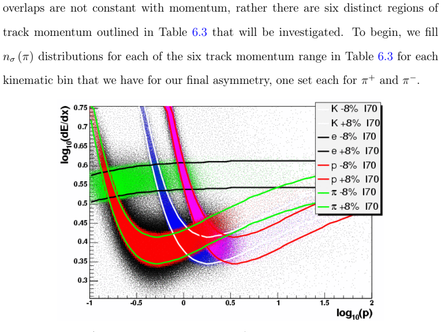
Studying Transverse Momentum Dependent Distributions in Polarized Proton Collisions Via Azimuthal Single Spin Asymmetries of Charged Pions in Jets
Pith reviewed 2026-05-24 16:19 UTC · model grok-4.3
The pith
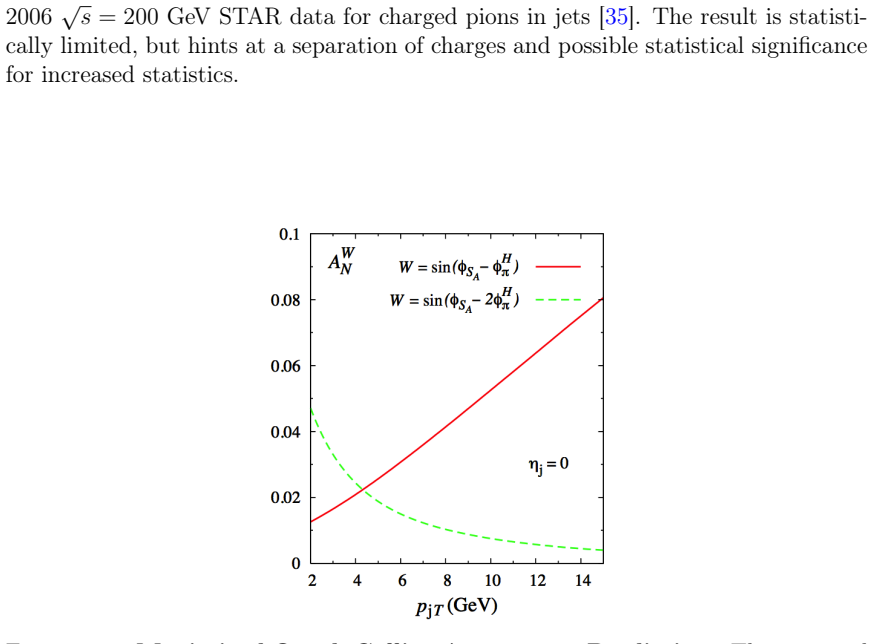
Azimuthal single spin asymmetries of charged pions in jets yield the first statistically significant Collins asymmetries from 200 GeV polarized proton collisions.
A machine-rendered reading of the paper's core claim, the machinery that carries it, and where it could break.
Core claim
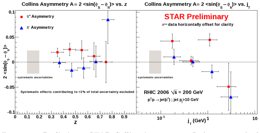
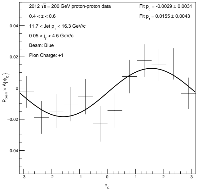
This thesis reports on the first statistically significant Collins asymmetries extracted from sqrt(s)=200 GeV hadronic collisions using 14 pb^{-1} of transversely polarized proton collisions at 57% average polarization. These asymmetries arise when the transversity distribution h1(x) couples to the Collins fragmentation function through spin-dependent azimuthal modulations of charged pions inside jets.
What carries the argument
Azimuthal single spin asymmetries of charged pions in jets, which isolate the product of transversity and the Collins fragmentation function in hadronic collisions.
If this is right
- The extracted asymmetries provide an independent data set that can be combined with SIDIS and e+e- results to tighten constraints on the transversity distribution h1(x).
- Hadronic collisions extend the accessible kinematic range in x and z beyond what is currently available from lepton-hadron scattering.
- The new channel allows direct study of transverse-momentum-dependent effects in a regime dominated by parton-parton scattering rather than virtual-photon exchange.
- Future higher-luminosity runs can test whether the measured asymmetries scale with beam polarization and integrated luminosity as predicted by the factorization framework.
Where Pith is reading between the lines
- Global analyses that incorporate these hadronic data points could reveal whether current tensions between different extractions of h1(x) arise from limited statistics or from process-dependent effects.
- The same jet-based technique could be applied to other final-state particles or to dijet observables to map additional transverse-momentum-dependent distributions.
- If the asymmetries persist at higher collision energies, they would offer a clean probe for testing the evolution of the Collins function with hard scale.
Load-bearing premise
The spin-dependent azimuthal distributions of charged pions in jets can isolate the Collins asymmetries without significant contamination from other spin-dependent effects or backgrounds in hadronic collisions.
What would settle it
A measurement in which the extracted azimuthal asymmetry is consistent with zero within statistical and systematic uncertainties after all background subtractions and corrections would falsify the claim of first statistically significant Collins asymmetries.
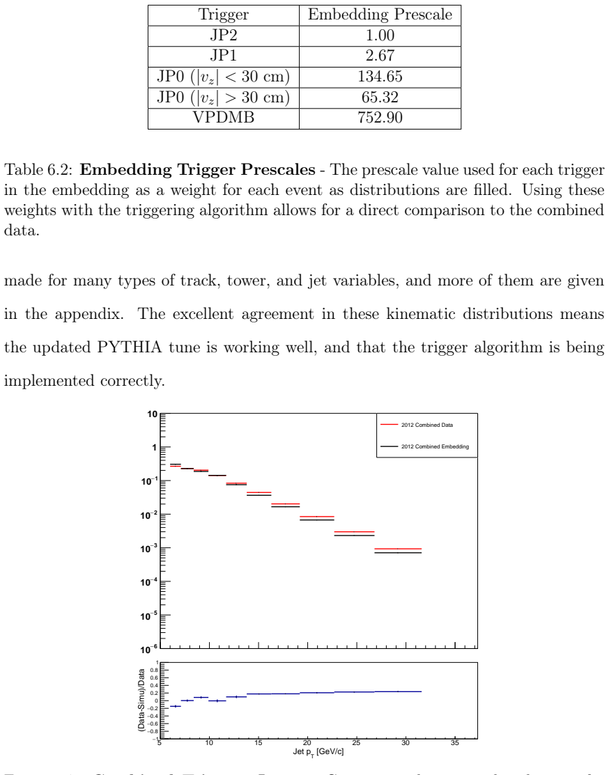
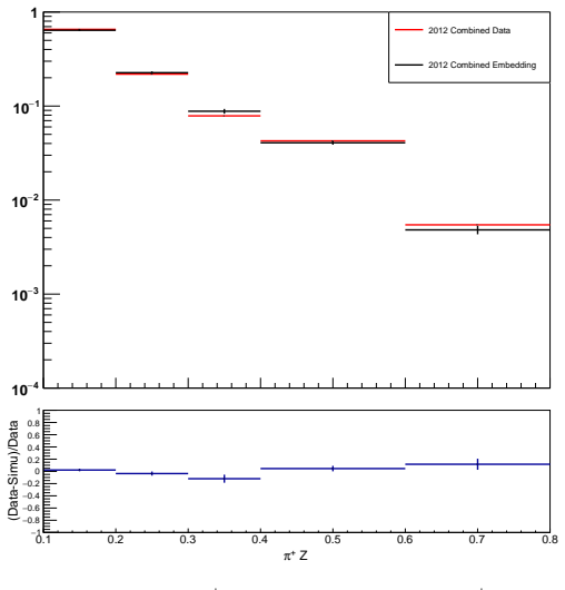
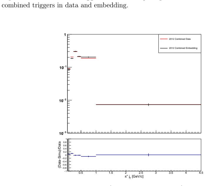
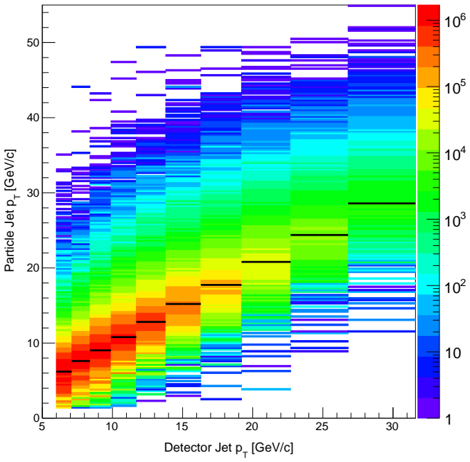
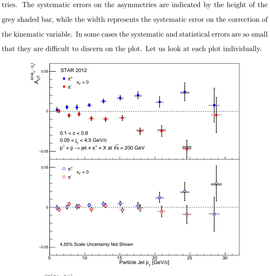
Figures
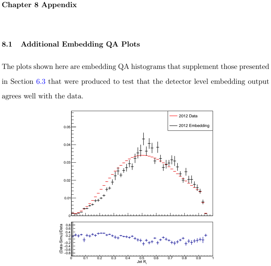
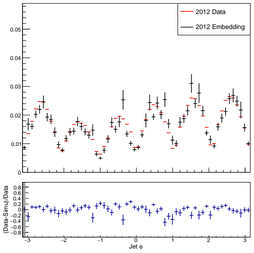

read the original abstract
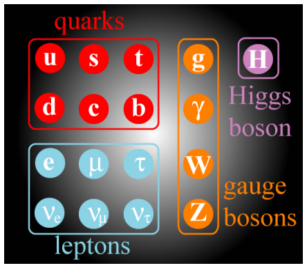
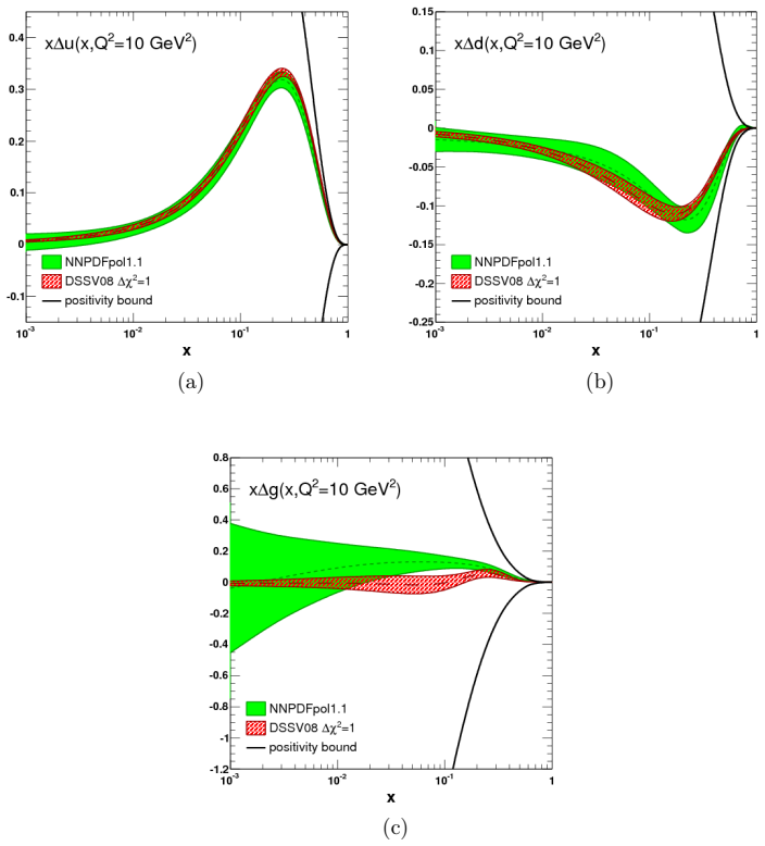
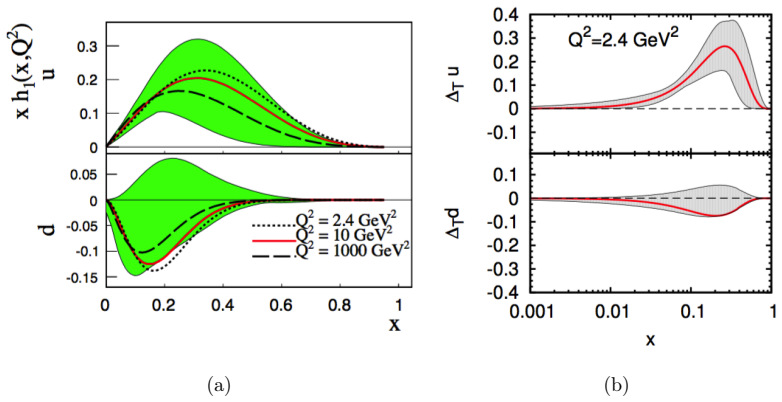
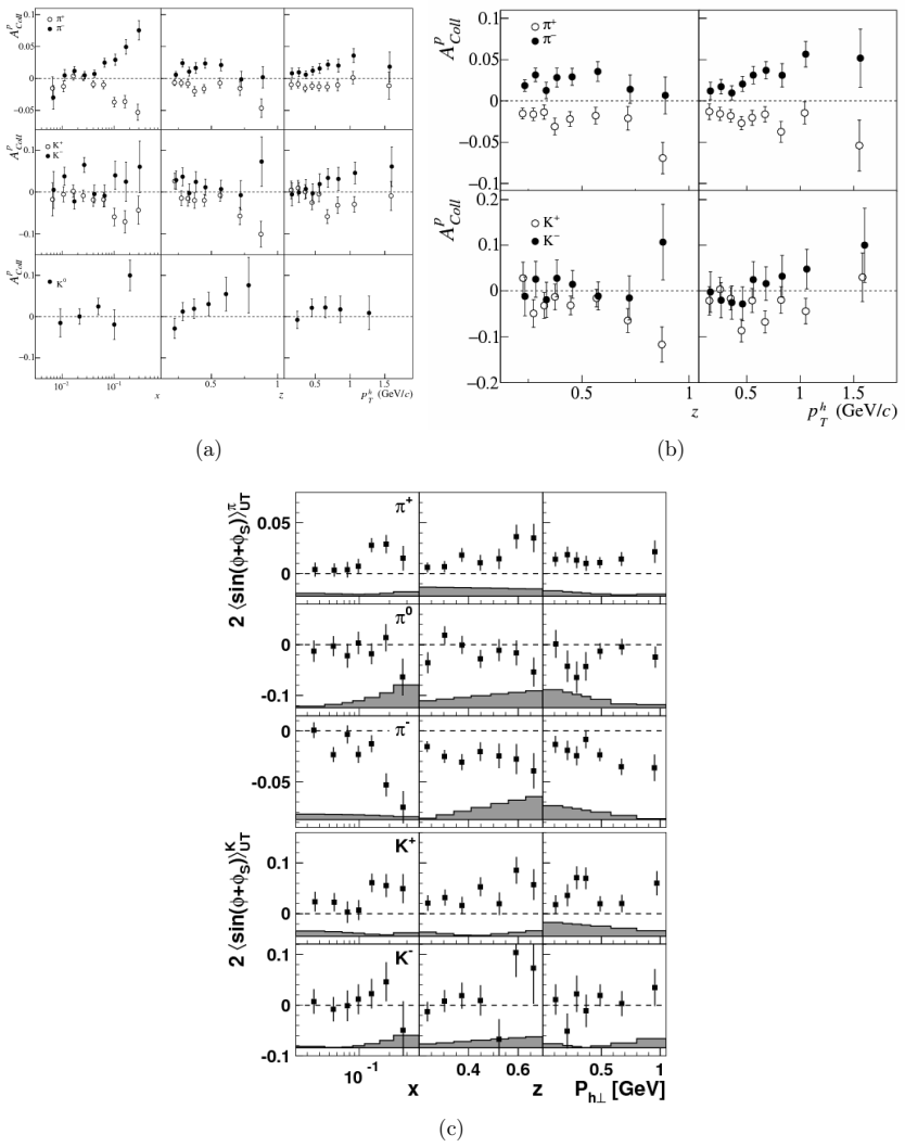
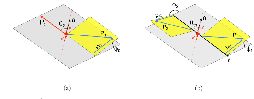
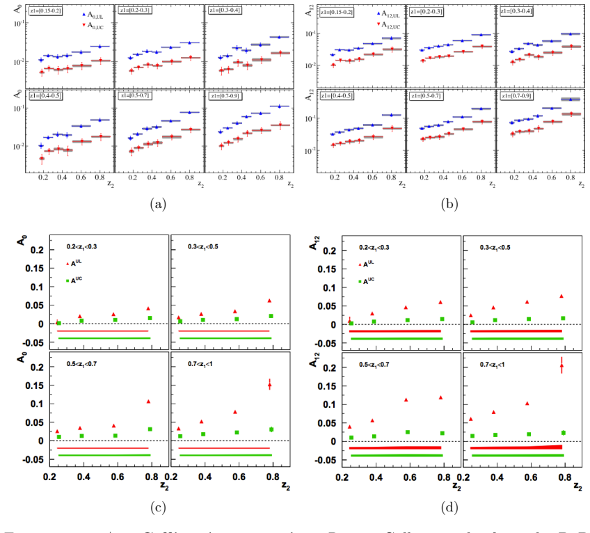
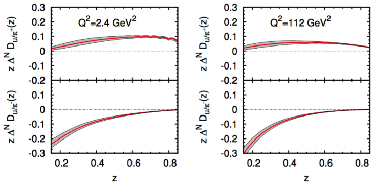
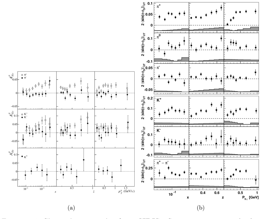
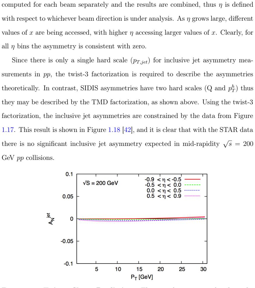
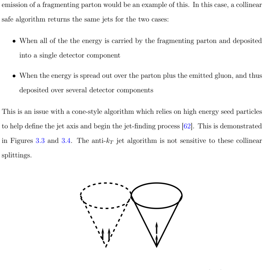
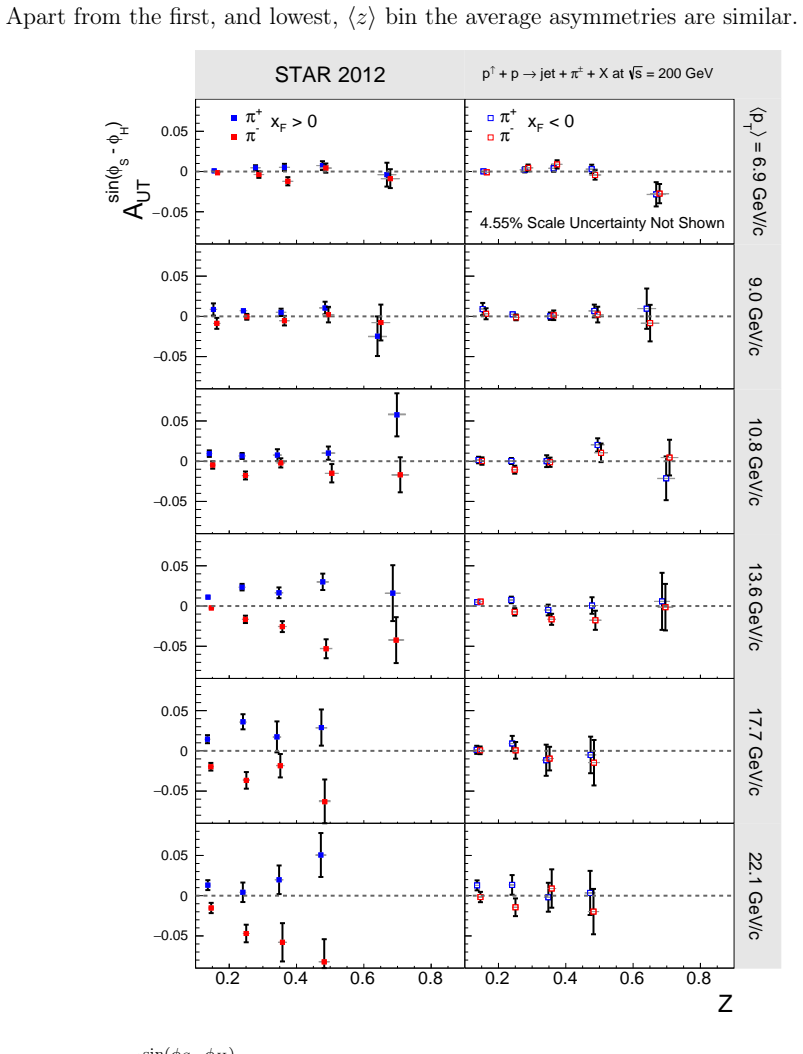
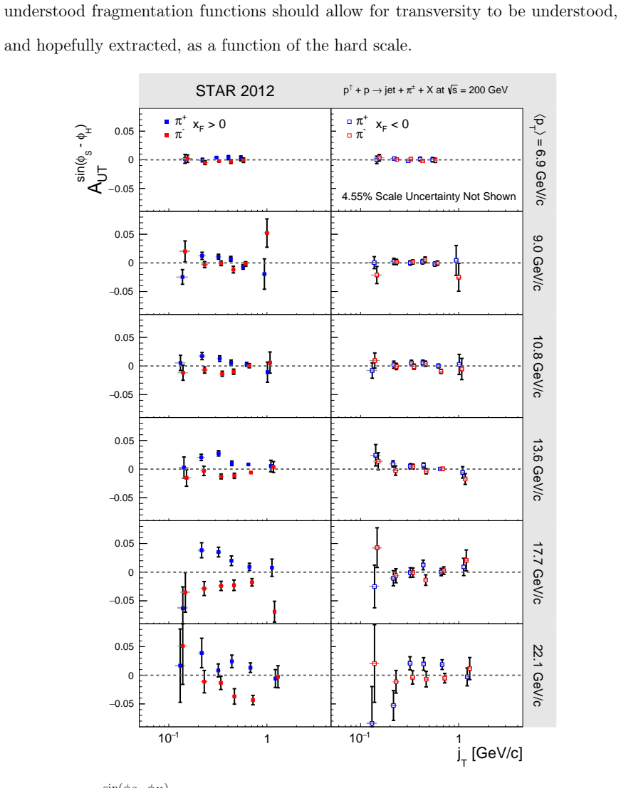
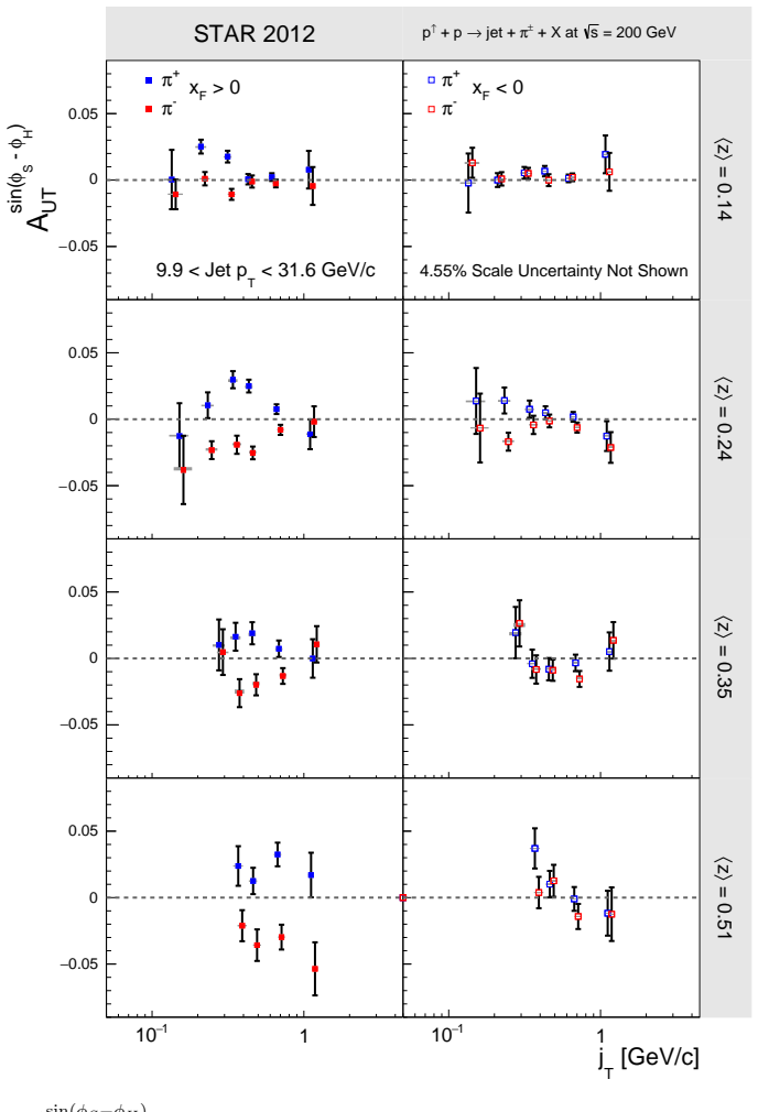
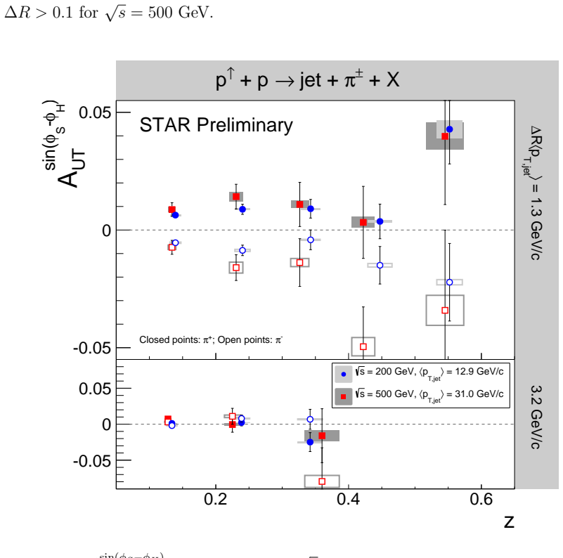
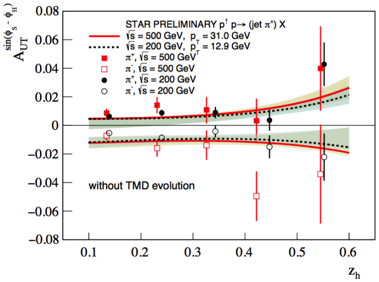
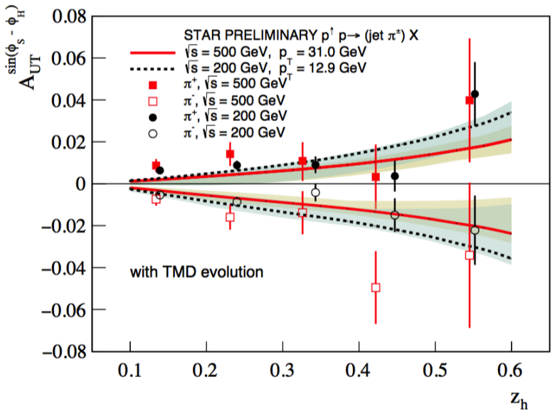
A complete, fundamental understanding of the proton must include knowledge of the underlying spin structure. The transversity distribution, $h_1\left(x\right)$, which describes the transverse spin structure of quarks inside of a transversely polarized proton, is only accessible through channels that couple $h_1 \left(x\right)$ to another chiral odd distribution, such as the Collins fragmentation function ($\Delta^N D_{\pi/q^\uparrow}\left(z,j_T\right)$). Significant Collins asymmetries of charged pions have been observed in semi-inclusive deep inelastic scattering (SIDIS) data. These SIDIS asymmetries combined with $e^+e^-$ process asymmetries have allowed for the extraction of $h_1\left(x\right)$ and $\Delta^N D_{\pi/q^\uparrow}\left(z,j_T\right)$. However, the current uncertainties on $h_1\left(x\right)$ are large compared to the corresponding quark momentum and helicity distributions and reflect the limited statistics and kinematic reach of the available data. In transversely polarized hadronic collisions, Collins asymmetries may be isolated and extracted by measuring the spin dependent azimuthal distributions of charged pions in jets. This thesis will report on the first statistically significant Collins asymmetries extracted from $\sqrt{s}=200$ GeV hadronic collisions using $14$ pb$^{-1}$ of transversely polarized proton collisions at 57% average polarization.
Editorial analysis
A structured set of objections, weighed in public.
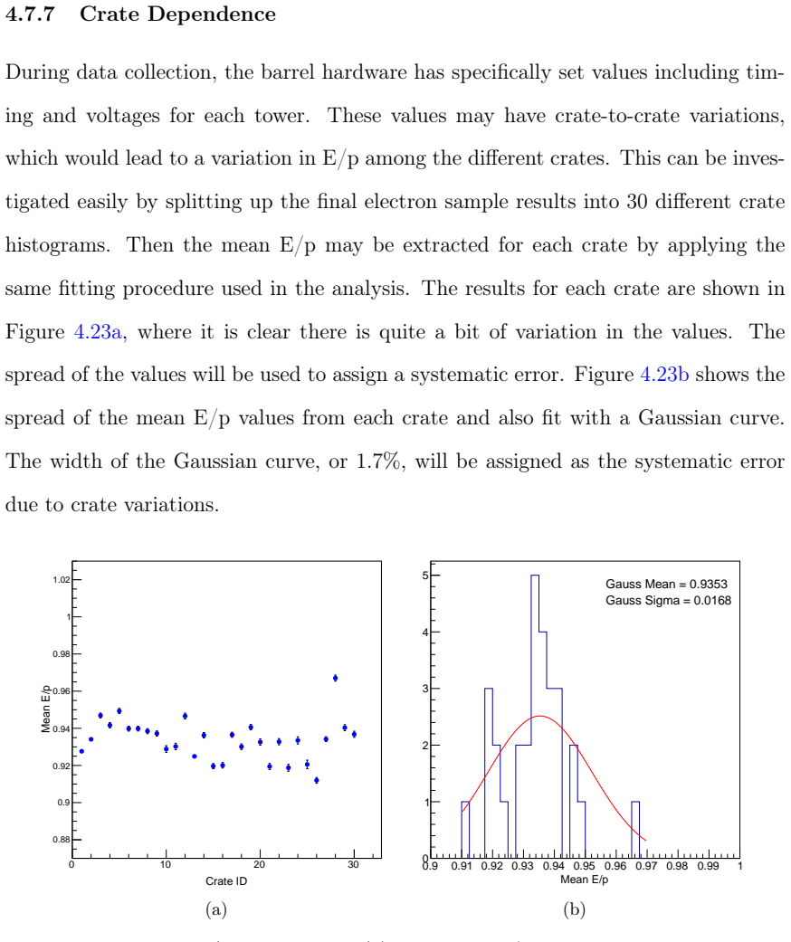
Referee Report
Summary. The manuscript reports the first extraction of statistically significant Collins asymmetries from azimuthal single-spin asymmetries of charged pions in jets produced in transversely polarized proton-proton collisions at √s=200 GeV. The analysis uses 14 pb^{-1} of data collected with an average beam polarization of 57% and isolates the asymmetries via spin-dependent azimuthal distributions to access the product of transversity h1(x) and the Collins fragmentation function.
Significance. If the central extraction holds, the result supplies the first Collins asymmetry data from hadronic collisions, extending the kinematic reach beyond existing SIDIS and e+e− measurements and offering new constraints on the transversity distribution with reduced uncertainties.
major comments (2)
- [Abstract] Abstract: the claim of the 'first statistically significant' extraction is stated without any reported asymmetry values, statistical significances, error bars, or systematic uncertainties. The results section must supply these quantities to substantiate the central claim of statistical significance.
- [Analysis] Analysis of azimuthal distributions: the isolation of the Collins contribution requires explicit quantitative demonstration that other spin-dependent effects and backgrounds do not produce significant contamination in the selected pion-in-jet sample; without such tests the interpretation remains vulnerable.
minor comments (1)
- [Abstract] The abstract would benefit from a concise statement of the observed asymmetry magnitudes to allow immediate assessment of the result's scale.
Simulated Author's Rebuttal
We thank the referee for the careful reading and constructive comments on our manuscript. We address each major comment below.
read point-by-point responses
-
Referee: [Abstract] Abstract: the claim of the 'first statistically significant' extraction is stated without any reported asymmetry values, statistical significances, error bars, or systematic uncertainties. The results section must supply these quantities to substantiate the central claim of statistical significance.
Authors: The results section presents the extracted Collins asymmetries for charged pions in jets, including central values, statistical and systematic uncertainties, and significances derived from the 14 pb^{-1} data set at 57% average polarization. To make the abstract claim self-contained and directly substantiated, we will revise the abstract to quote the key measured asymmetries and their significances. revision: yes
-
Referee: [Analysis] Analysis of azimuthal distributions: the isolation of the Collins contribution requires explicit quantitative demonstration that other spin-dependent effects and backgrounds do not produce significant contamination in the selected pion-in-jet sample; without such tests the interpretation remains vulnerable.
Authors: The analysis isolates the Collins term via the spin-dependent azimuthal modulation in the pion-in-jet sample and includes consistency checks across kinematic bins and comparisons to unpolarized reference samples to constrain other contributions. To meet the request for explicit quantitative demonstration, we will add a dedicated subsection with numerical estimates (including upper limits) on residual contamination from other spin-dependent effects and backgrounds. revision: yes
Circularity Check
No significant circularity in experimental measurement report
full rationale
This document is an experimental thesis reporting the extraction of Collins asymmetries from 14 pb^{-1} of √s=200 GeV transversely polarized p+p collision data. The abstract and described content contain no derivation chain, no fitted parameters renamed as predictions, no self-citation load-bearing uniqueness theorems, and no ansatz smuggling. The central claim rests on direct analysis of collected collision data rather than any reduction of outputs to inputs by construction. No load-bearing steps reduce to self-referential definitions or prior fitted quantities.
Axiom & Free-Parameter Ledger
axioms (1)
- domain assumption The Collins fragmentation function couples to transversity in hadronic collisions in the same way as in SIDIS
Lean theorems connected to this paper
-
IndisputableMonolith/Foundation/RealityFromDistinction.leanreality_from_one_distinction unclear?
unclearRelation between the paper passage and the cited Recognition theorem.
This thesis will report on the first statistically significant Collins asymmetries extracted from √s=200 GeV hadronic collisions using 14 pb^{-1} of transversely polarized proton collisions at 57% average polarization.
-
IndisputableMonolith/Cost/FunctionalEquation.leanwashburn_uniqueness_aczel unclear?
unclearRelation between the paper passage and the cited Recognition theorem.
Collins asymmetries may be isolated and extracted by measuring the spin dependent azimuthal distributions of charged pions in jets.
What do these tags mean?
- matches
- The paper's claim is directly supported by a theorem in the formal canon.
- supports
- The theorem supports part of the paper's argument, but the paper may add assumptions or extra steps.
- extends
- The paper goes beyond the formal theorem; the theorem is a base layer rather than the whole result.
- uses
- The paper appears to rely on the theorem as machinery.
- contradicts
- The paper's claim conflicts with a theorem or certificate in the canon.
- unclear
- Pith found a possible connection, but the passage is too broad, indirect, or ambiguous to say the theorem truly supports the claim.
Reference graph
Works this paper leans on
-
[1]
Magnetic Deviation of Hydrogen Molecules and the Magnetic Moment of the Proton. I.,
R. Frisch and O. Stern, “Magnetic Deviation of Hydrogen Molecules and the Magnetic Moment of the Proton. I.,”Z. Phys., vol. 85, pp. 4–16, 1933
work page 1933
-
[2]
Magnetic Deviation of Hydrogen Molecules and the Magnetic Moment of the Proton. II.,
I. Esterman and O. Stern, “Magnetic Deviation of Hydrogen Molecules and the Magnetic Moment of the Proton. II.,”Z. Phys., vol. 85, pp. 17–24, 1933
work page 1933
-
[3]
Shankar, Principles of Quantum Mechanics
R. Shankar, Principles of Quantum Mechanics. Springer, 2nd ed., 1994
work page 1994
-
[4]
Griffiths, Introduction to Elementary Particles
D. Griffiths, Introduction to Elementary Particles. Wiley-VCH, 2nd ed., 2008
work page 2008
-
[5]
P. Skands, “Introduction to QCD,” in Proceedings, Theoretical Advanced Study Institute in Elementary Particle Physics: Searching for New Physics at Small and Large Scales (TASI 2012), pp. 341–420, 2013
work page 2012
-
[6]
A. Ali and G. Kramer, “Jets and QCD: A Historical Review of the Discovery of the Quark and Gluon Jets and its Impact on QCD,”Eur. Phys. J., vol. H36, pp. 245–326, 2011
work page 2011
-
[7]
Prospects for spin physics at RHIC,
G. Bunce, N. Saito, J. Soffer, and W. Vogelsang, “Prospects for spin physics at RHIC,” Ann. Rev. Nucl. Part. Sci., vol. 50, pp. 525–575, 2000
work page 2000
-
[8]
The RHIC Cold QCD Plan for 2017 to 2023: A Portal to the EIC,
E.-C. Aschenauer et al., “The RHIC Cold QCD Plan for 2017 to 2023: A Portal to the EIC,” 2016
work page 2017
-
[9]
Pitonyak, Exploring the Structure of Hadrons Through Spin Asymmetries in Hard Scattering Processes
D. Pitonyak, Exploring the Structure of Hadrons Through Spin Asymmetries in Hard Scattering Processes. PhD thesis, Temple University, May 2013
work page 2013
-
[10]
A Unified picture for sin- gle transverse-spin asymmetries in hard processes,
X. Ji, J.-W. Qiu, W. Vogelsang, and F. Yuan, “A Unified picture for sin- gle transverse-spin asymmetries in hard processes,” Phys. Rev. Lett., vol. 97, p. 082002, 2006
work page 2006
-
[11]
Transverse polarisation of quarks in hadrons,
V. Barone, A. Drago, and P. G. Ratcliffe, “Transverse polarisation of quarks in hadrons,” Phys. Rept., vol. 359, pp. 1–168, 2002
work page 2002
-
[12]
Single Spin Production Asymmetries from the Hard Scattering of Point-Like Constituents,
D. W. Sivers, “Single Spin Production Asymmetries from the Hard Scattering of Point-Like Constituents,”Phys. Rev., vol. D41, p. 83, 1990
work page 1990
-
[13]
Time reversal odd distribution functions in lepto- production,
D. Boer and P. J. Mulders, “Time reversal odd distribution functions in lepto- production,” Phys. Rev., vol. D57, pp. 5780–5786, 1998
work page 1998
-
[14]
H. Avakian, A. V. Efremov, P. Schweitzer, and F. Yuan, “Transverse mo- mentum dependent distribution function h⊥ 1T and the single spin asymmetry AUT sin (3φ− φS),” Phys. Rev., vol. D78, p. 114024, 2008
work page 2008
-
[15]
G. A. Miller, “Shapes of the proton,”Phys. Rev., vol. C68, p. 022201, 2003. 210
work page 2003
-
[16]
L. L. Pappalardo, “Accessing TMDs at HERMES,”AIP Conf. Proc., vol. 1441, pp. 229–232, 2012
work page 2012
-
[17]
Azimuthal asymmetries for hadron distributions inside a jet in hadronic collisions,
U. D’Alesio, F. Murgia, and C. Pisano, “Azimuthal asymmetries for hadron distributions inside a jet in hadronic collisions,”Phys. Rev., vol. D83, p. 034021, 2011
work page 2011
-
[18]
Fragmentation of transversely polarized quarks probed in trans- verse momentum distributions,
J. C. Collins, “Fragmentation of transversely polarized quarks probed in trans- verse momentum distributions,”Nucl. Phys., vol. B396, pp. 161–182, 1993
work page 1993
-
[19]
J. Collins and T. Rogers, “Understanding the large-distance behavior of transverse-momentum-dependent parton densities and the Collins-Soper evolu- tion kernel,”Phys. Rev., vol. D91, no. 7, p. 074020, 2015
work page 2015
-
[21]
Y. L. Dokshitzer, “Calculation of the Structure Functions for Deep Inelastic Scattering and e+ e- Annihilation by Perturbation Theory in Quantum Chro- modynamics.,” Sov. Phys. JETP, vol. 46, pp. 641–653, 1977. [Zh. Eksp. Teor. Fiz.73,1216(1977)]
work page 1977
-
[22]
Deep inelastic e p scattering in perturbation theory,
V. N. Gribov and L. N. Lipatov, “Deep inelastic e p scattering in perturbation theory,” Sov. J. Nucl. Phys., vol. 15, pp. 438–450, 1972. [Yad. Fiz.15,781(1972)]
work page 1972
-
[23]
Asymptotic Freedom in Parton Language,
G. Altarelli and G. Parisi, “Asymptotic Freedom in Parton Language,”Nucl. Phys., vol. B126, pp. 298–318, 1977
work page 1977
-
[24]
H. Abramowiczet al., “Combination of measurements of inclusive deep inelastic e±p scattering cross sections and QCD analysis of HERA data,”Eur. Phys. J., vol. C75, no. 12, p. 580, 2015
work page 2015
-
[25]
A first unbiased global determination of polarized PDFs and their uncertainties,
E. R. Nocera, R. D. Ball, S. Forte, G. Ridolfi, and J. Rojo, “A first unbiased global determination of polarized PDFs and their uncertainties,”Nucl. Phys., vol. B887, pp. 276–308, 2014
work page 2014
-
[26]
Z.-B. Kang, A. Prokudin, P. Sun, and F. Yuan, “Extraction of Quark Transver- sity Distribution and Collins Fragmentation Functions with QCD Evolution,” Phys. Rev., vol. D93, no. 1, p. 014009, 2016
work page 2016
-
[27]
M. Anselmino, M. Boglione, U. D’Alesio, J. O. Gonzalez Hernandez, S. Melis, F. Murgia, and A. Prokudin, “Collins functions for pions from SIDIS and new e+e− data: a first glance at their transverse momentum dependence,”Phys. Rev., vol. D92, no. 11, p. 114023, 2015
work page 2015
-
[28]
Extraction of Spin- Dependent Parton Densities and Their Uncertainties,
D. de Florian, R. Sassot, M. Stratmann, and W. Vogelsang, “Extraction of Spin- Dependent Parton Densities and Their Uncertainties,” Phys. Rev., vol. D80, p. 034030, 2009. 211
work page 2009
-
[29]
Semi-inclusive deep inelastic scattering at small transverse momentum,
A. Bacchetta, M. Diehl, K. Goeke, A. Metz, P. J. Mulders, and M. Schlegel, “Semi-inclusive deep inelastic scattering at small transverse momentum,”JHEP, vol. 02, p. 093, 2007
work page 2007
-
[30]
Single-spin asymmetries: The Trento conventions,
A. Bacchetta, U. D’Alesio, M. Diehl, and C. A. Miller, “Single-spin asymmetries: The Trento conventions,”Phys. Rev., vol. D70, p. 117504, 2004
work page 2004
-
[31]
C. Adolph et al., “Collins and Sivers asymmetries in muonproduction of pions and kaons offtransversely polarised protons,”Phys. Lett., vol. B744, pp. 250–259, 2015
work page 2015
-
[32]
Effects of transversity in deep-inelastic scattering by po- larized protons,
A. Airapetian et al., “Effects of transversity in deep-inelastic scattering by po- larized protons,”Phys. Lett., vol. B693, pp. 11–16, 2010
work page 2010
-
[33]
J. P. Leeset al., “Measurement of Collins asymmetries in inclusive production of charged pion pairs ine+e− annihilation at BABAR,”Phys. Rev., vol. D90, no. 5, p. 052003, 2014
work page 2014
-
[34]
R. Seidlet al., “Measurement of Azimuthal Asymmetries in Inclusive Production of Hadron Pairs ine+e− Annihilation at√s = 10.58 GeV,”Phys. Rev., vol. D78, p. 032011, 2008. [Erratum: Phys. Rev.D86,039905(2012)]
work page 2008
-
[35]
Constraining Quark Transversity through Collins Asymmetry Mea- surements at STAR,
R. Fatemi, “Constraining Quark Transversity through Collins Asymmetry Mea- surements at STAR,”AIP Conf. Proc., vol. 1441, pp. 233–237, 2012
work page 2012
-
[36]
New insight on the Sivers transverse momentum dependent distribution func- tion,
M. Anselmino, M. Boglione, U. D’Alesio, S. Melis, F. Murgia, and A. Prokudin, “New insight on the Sivers transverse momentum dependent distribution func- tion,” J. Phys. Conf. Ser., vol. 295, p. 012062, 2011
work page 2011
-
[37]
Observation of the Naive-T-odd Sivers Effect in Deep- Inelastic Scattering,
A. Airapetian et al., “Observation of the Naive-T-odd Sivers Effect in Deep- Inelastic Scattering,”Phys. Rev. Lett., vol. 103, p. 152002, 2009
work page 2009
-
[38]
Sivers Effect for Pion and Kaon Production in Semi- Inclusive Deep Inelastic Scattering,
M. Anselmino, M. Boglione, U. D’Alesio, A. Kotzinian, S. Melis, F. Murgia, A. Prokudin, and C. Turk, “Sivers Effect for Pion and Kaon Production in Semi- Inclusive Deep Inelastic Scattering,”Eur. Phys. J., vol. A39, pp. 89–100, 2009
work page 2009
-
[39]
QCD asymmetry and polarized hadron structure function measurement,
A. V. Efremov and O. V. Teryaev, “QCD asymmetry and polarized hadron structure function measurement,”Physics Letters B, vol. 150, pp. 383–386, Jan. 1985
work page 1985
-
[40]
Single transverse spin asymmetries,
J. Qiu and G. Sterman, “Single transverse spin asymmetries,”Phys. Rev. Lett., vol. 67, pp. 2264–2267, Oct 1991
work page 1991
-
[41]
L. Adamczyket al., “Longitudinal and transverse spin asymmetries for inclusive jet production at mid-rapidity in polarizedp + p collisions at√s = 200 GeV,” Phys. Rev., vol. D86, p. 032006, 2012
work page 2012
-
[42]
Single transverse-spin asymmetry for direct-photon and single-jet productions at RHIC,
K. Kanazawa and Y. Koike, “Single transverse-spin asymmetry for direct-photon and single-jet productions at RHIC,”Phys. Lett., vol. B720, pp. 161–165, 2013. 212
work page 2013
-
[43]
Optically pumped polarized h-ion source for rhic spin physics,
A. Zelenski, J. Alessi, B. Briscoe, G. Dutto, H. Huang, A. Kponou, S. Kokhanovski, V. Klenov, A. Lehrach, P. Levy, et al., “Optically pumped polarized h-ion source for rhic spin physics,”Review of scientific instruments, vol. 73, no. 2, pp. 888–891, 2002
work page 2002
-
[44]
Accelerating Polarized Protons to High Energy,
M. Bai, “Accelerating Polarized Protons to High Energy,” Conf. Proc., vol. C100523, p. THPPMH01, 2010
work page 2010
-
[45]
Alekseevet al., Configuration manual polarized proton collider at RHIC, 2012
I. Alekseevet al., Configuration manual polarized proton collider at RHIC, 2012
work page 2012
-
[46]
Commissioning of RHIC p carbon CNI polarimeter,
H. Huang et al., “Commissioning of RHIC p carbon CNI polarimeter,” Nucl. Phys., vol. A721, pp. 356–359, 2003. [,795(2000)]
work page 2003
-
[47]
AbsolutepolarizedH-jetpolarimeterdevelopment, forRHIC,
A.Zelenski et al., “AbsolutepolarizedH-jetpolarimeterdevelopment, forRHIC,” Nucl. Instrum. Meth., vol. A536, pp. 248–254, 2005
work page 2005
-
[48]
K. H. Ackermann et al., “STAR detector overview,” Nucl. Instrum. Meth., vol. A499, pp. 624–632, 2003
work page 2003
-
[49]
T. Sakuma,Inclusive Jet and Dijet Production in Polarized Proton-Proton Col- lisions at√s = 200 GeV at RHIC. PhD thesis, Massachusetts Institute of Technology, 2010
work page 2010
-
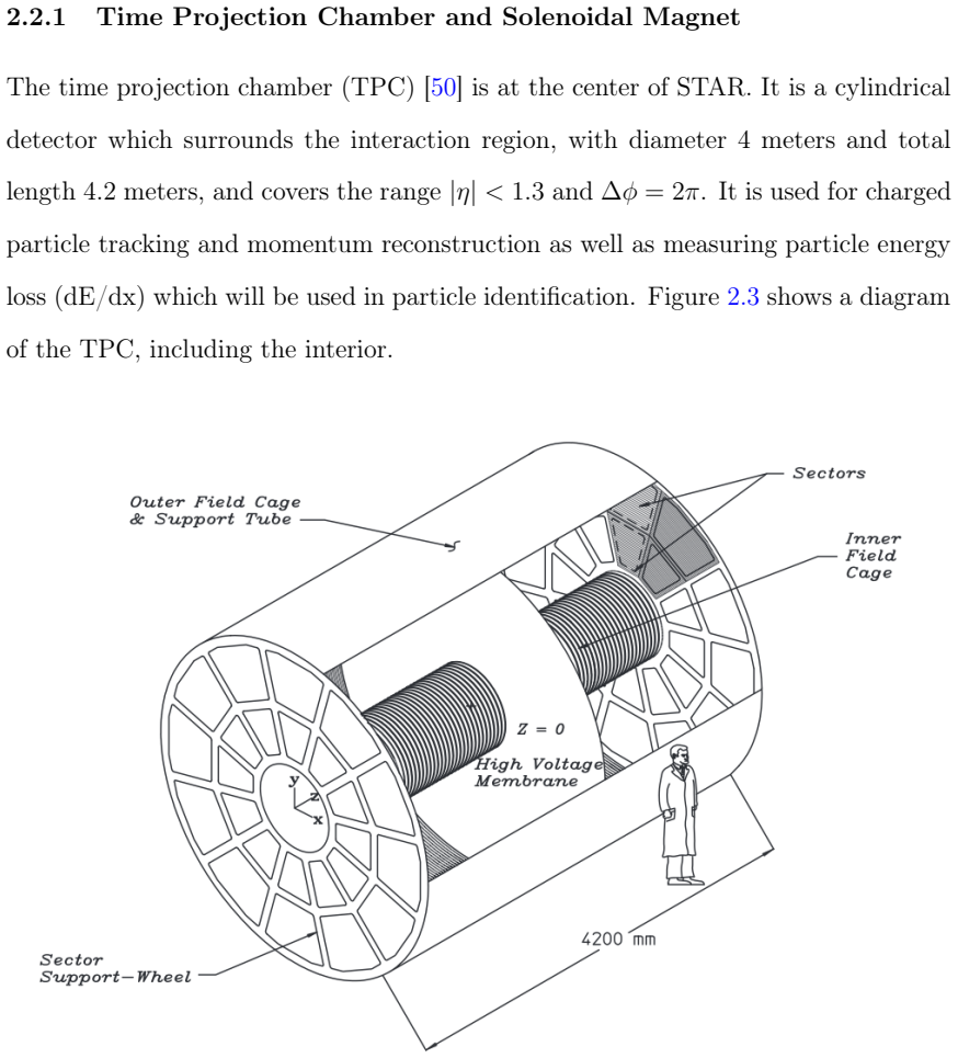
[50]
The Star time projection chamber: A Unique tool for studying high multiplicity events at RHIC,
M. Anderson et al., “The Star time projection chamber: A Unique tool for studying high multiplicity events at RHIC,”Nucl. Instrum. Meth., vol. A499, pp. 659–678, 2003
work page 2003
-
[51]
L. Kochenda, S. Kozlov, P. Kravtsov, A. Markov, M. Strikhanov, B. Stringfellow, V. Trofimov, R. Wells, and H. Wieman, “STAR TPC gas system,”Nucl. Instrum. Meth., vol. A499, pp. 703–712, 2003
work page 2003
-
[52]
The STAR detector magnet subsystem,
F. Bergsma et al., “The STAR detector magnet subsystem,” Nucl. Instrum. Meth., vol. A499, pp. 633–639, 2003
work page 2003
-
[53]
K. A. Oliveet al., “Review of Particle Physics,”Chin. Phys., vol. C38, p. 090001, 2014
work page 2014
-
[54]
Extensive particle identification with TPC and TOF at the STAR experiment,
M. Shao et al., “Extensive particle identification with TPC and TOF at the STAR experiment,”Nucl. Instrum. Meth., vol. A558, pp. 419–429, 2006
work page 2006
-
[55]
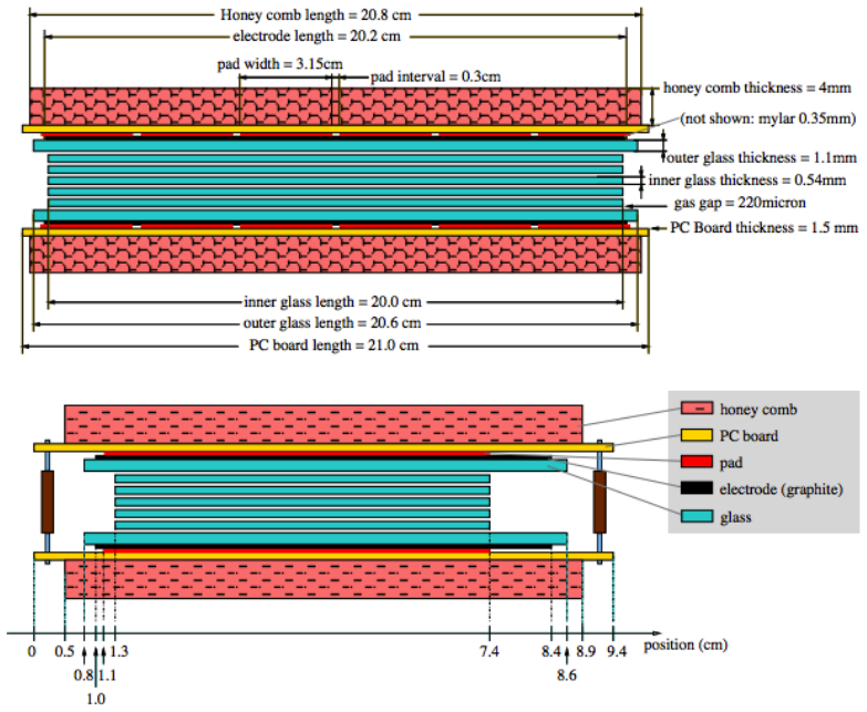
The STAR barrel electromagnetic calorimeter,
M. Beddoet al., “The STAR barrel electromagnetic calorimeter,”Nucl. Instrum. Meth., vol. A499, pp. 725–739, 2003
work page 2003
-
[56]
The star endcap electromagnetic calorimeter,
C. Allgoweret al., “The star endcap electromagnetic calorimeter,”Nuclear In- struments and Methods in Physics Research Section A: Accelerators, Spectrom- eters, Detectors and Associated Equipment, vol. 499, no. 2, pp. 740–750, 2003
work page 2003
-
[57]
The STAR Vertex Position Detector,
W. J. Llopeet al., “The STAR Vertex Position Detector,”Nucl. Instrum. Meth., vol. A759, pp. 23–28, 2014. 213
work page 2014
-
[58]
Proposal for a Large Area Time of Flight System for STAR
STAR TOF Collaboration, “Proposal for a Large Area Time of Flight System for STAR.” Local analysis note, 2004
work page 2004
-
[59]
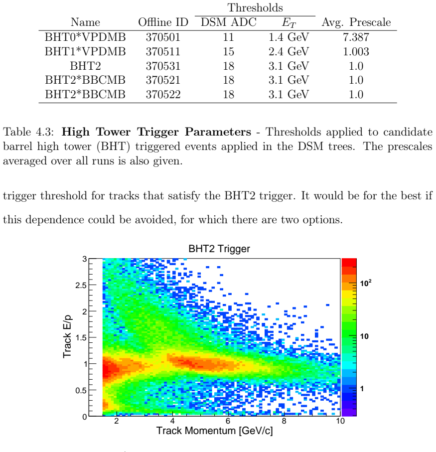
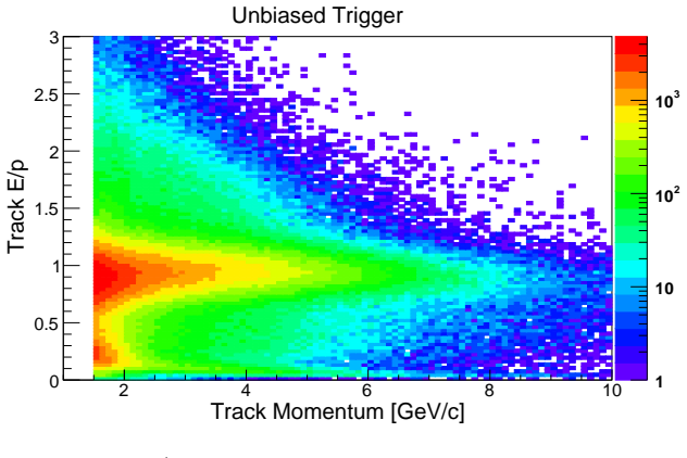
F. Bieseret al., “The STAR trigger,”Nucl. Instrum. Meth. A, vol. 499, pp. 766– 777, March 2003
work page 2003
-
[60]
M. Cacciari, G. P. Salam, and G. Soyez, “FastJet User Manual,”Eur.Phys.J., vol. C72, p. 1896, 2012
work page 2012
-
[61]
The Anti-kT jet clustering algorithm,
M. Cacciari, G. P. Salam, and G. Soyez, “The Anti-kT jet clustering algorithm,” JHEP, vol. 0804, p. 063, 2008
work page 2008
-
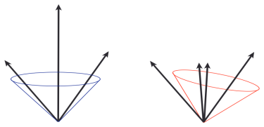
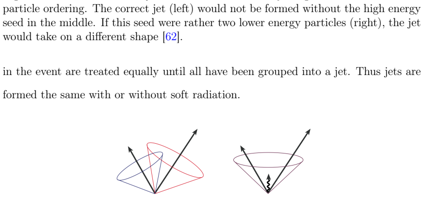
[62]
G. C. Blazey, J. R. Dittmann, S. Ellis, V. D. Elvira, K. Frame,et al., “Run II jet physics,” Proceedings of QCD and weak boson physics in Run II, pp. 47–77, 2000
work page 2000
-
[63]
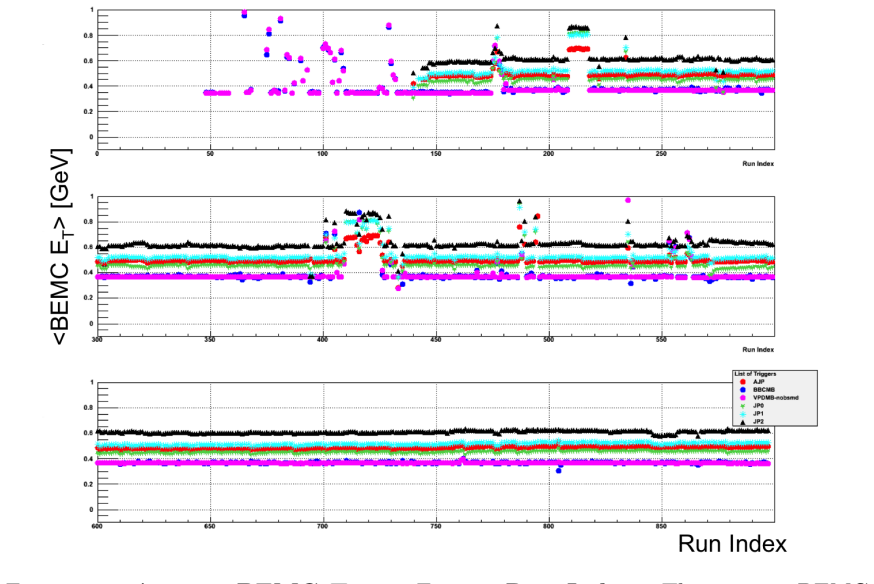
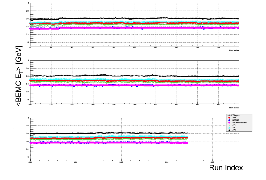
2006 BEMC Tower Calibration Report
M. Betancourt, A. Hoffman, A. Kocoloski, and M. Walker, “2006 BEMC Tower Calibration Report.” Local analysis note, 2009
work page 2006
-
[64]
Leo, Techniques for Nuclear and Particle Physics Experiments, vol
W. Leo, Techniques for Nuclear and Particle Physics Experiments, vol. 1 of1. Springer-Verlag Berlin Heidelberg, 2 ed., 2 1994
work page 1994
-
[65]
ROOT: An object oriented data analysis frame- work,
R. Brun and F. Rademakers, “ROOT: An object oriented data analysis frame- work,” Nucl. Instrum. Meth., vol. A389, pp. 81–86, 1997
work page 1997
-
[66]
Collins azimuthal asymme- tries of hadron production inside jets,
Z.-B. Kang, A. Prokudin, F. Ringer, and F. Yuan, “Collins azimuthal asymme- tries of hadron production inside jets,”ArXiv e-prints, July 2017
work page 2017
-
[67]
Techniques for measurement of spin-1/2 and spin-1 polarization analyzing tensors,
G. G. Ohlsen and P. W. Keaton, “Techniques for measurement of spin-1/2 and spin-1 polarization analyzing tensors,”Nucl. Instrum. Meth., vol. 109, pp. 41–59, 1973
work page 1973
-
[68]
PYTHIA 6.4 Physics and Manual,
T. Sjostrand, S. Mrenna, and P. Z. Skands, “PYTHIA 6.4 Physics and Manual,” JHEP, vol. 05, p. 026, 2006
work page 2006
-
[69]
R. Brun, F. Bruyant, M. Maire, A. C. McPherson, and P. Zanarini, “GEANT3,” 1987
work page 1987
-
[70]
J. Adams et al., “Pion, kaon, proton and anti-proton transverse momentum distributions from p + p and d+ Au collisions at√sNN = 200GeV,” Phys. Lett., vol. B616, pp. 8–16, 2005
work page 2005
-
[71]
G. Agakishiev et al., “Identified hadron compositions in p+p and Au+Au col- lisions at high transverse momenta at√sN N = 200 GeV,” Phys. Rev. Lett., vol. 108, p. 072302, 2012
work page 2012
-
[72]
L. Adamczyk et al., “Precision Measurement of the Longitudinal Double-spin Asymmetry for Inclusive Jet Production in Polarized Proton Collisions at√s = 200 GeV,” Phys. Rev. Lett., vol. 115, no. 9, p. 092002, 2015. 214
work page 2015
-
[73]
Tuning Monte Carlo Generators: The Perugia Tunes,
P. Z. Skands, “Tuning Monte Carlo Generators: The Perugia Tunes,”Phys. Rev., vol. D82, p. 074018, 2010
work page 2010
-
[74]
The underlying event in large transverse momentum charged jet and Z− boson production,
R. Field, “The underlying event in large transverse momentum charged jet and Z− boson production,” Int. J. Mod. Phys., vol. A16S1A, pp. 250–254, 2001
work page 2001
-
[75]
Charged jet evolution and the underlying event inp¯pcollisions at 1.8 TeV,
T. Affolderet al., “Charged jet evolution and the underlying event inp¯pcollisions at 1.8 TeV,”Phys. Rev., vol. D65, p. 092002, 2002
work page 2002
-
[76]
The Underlying event in hard scattering processes,
R. D. Field, “The Underlying event in hard scattering processes,” eConf, vol. C010630, p. P501, 2001
work page 2001
-
[77]
The underlying event in hard interactions at the Tevatron¯pp collider,
D. Acostaet al., “The underlying event in hard interactions at the Tevatron¯pp collider,” Phys. Rev., vol. D70, p. 072002, 2004
work page 2004
-
[78]
Min-bias and the underlying event in Run 2 at CDF,
R. Field, “Min-bias and the underlying event in Run 2 at CDF,”Acta Phys. Polon., vol. B36, pp. 167–178, 2005
work page 2005
-
[79]
Measurement of the Underlying Event at Tevatron,
D. Kar, “Measurement of the Underlying Event at Tevatron,” inQCD and high energy interactions. Proceedings, 44th Rencontres de Moriond, La Thuile, Italy, March 14-21, 2009, pp. 277–280, 2009
work page 2009
-
[80]
New generation of parton distributions with uncertainties from global QCD analysis,
J. Pumplin, D. R. Stump, J. Huston, H. L. Lai, P. M. Nadolsky, and W. K. Tung, “New generation of parton distributions with uncertainties from global QCD analysis,”JHEP, vol. 07, p. 012, 2002
work page 2002
-
[81]
L. Huo, “In-Jet Tracking Efficiency Analysis for the STAR Time Projection Chamber in Polarized Proton-Proton Collisions at√s = 200 GeV,” Master’s thesis, Texas A&M University, May 2012
work page 2012
discussion (0)
Sign in with ORCID, Apple, or X to comment. Anyone can read and Pith papers without signing in.