Unit Averaging for Heterogeneous Panels
Pith reviewed 2026-05-24 11:11 UTC · model grok-4.3
The pith
A weighted average of all unit estimators recovers each unit's parameter with lower error in heterogeneous panels.
A machine-rendered reading of the paper's core claim, the machinery that carries it, and where it could break.
Core claim
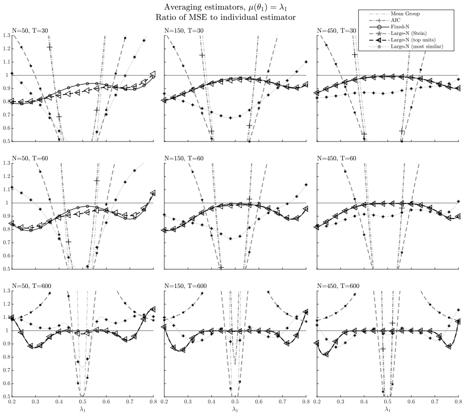
The authors introduce a unit averaging procedure to recover unit-specific parameters in a heterogeneous panel model. The procedure estimates the parameter of a given unit using a weighted average of all the unit-specific parameter estimators in the panel. The weights are determined by minimizing an MSE criterion derived in the paper. In a local heterogeneity framework inspired by frequentist model averaging, the local asymptotic distribution of the minimum MSE unit averaging estimator and the corresponding weights is derived. Benefits are illustrated with an application to forecasting unemployment rates for a panel of German regions.
What carries the argument
The minimum MSE unit averaging estimator, a weighted average of all unit-specific estimators whose weights minimize the derived mean squared error criterion under the local heterogeneity framework.
If this is right
- The averaged estimator attains a lower local asymptotic MSE than the individual unit estimator when heterogeneity is local.
- The optimal weights converge to values that reflect the relative bias-variance trade-off across units.
- The local asymptotic distribution supplies a basis for constructing confidence intervals for the recovered unit parameters.
- Forecast accuracy for regional unemployment rates improves relative to separate estimation in the German panel application.
Where Pith is reading between the lines
- The same weighting logic could be applied to other panel settings such as firm-level or country-level data with moderate differences across units.
- Combining unit averaging with existing shrinkage or regularization methods might further reduce error in high-dimensional panels.
- If heterogeneity turns out to be stronger than the local framework assumes, separate estimation may remain preferable and the method would require extension.
- A simulation exercise that varies the heterogeneity parameter continuously could map the range where averaging dominates individual estimation.
Load-bearing premise
The local heterogeneity framework holds and permits derivation of the local asymptotic distribution of the estimator and the corresponding weights.
What would settle it
A Monte Carlo experiment or real panel dataset in which the mean squared error of the unit averaging estimator exceeds the mean squared error of the separate unit estimator under moderate local heterogeneity would refute the efficiency gain.
Figures


read the original abstract
In this work we introduce a unit averaging procedure to efficiently recover unit-specific parameters in a heterogeneous panel model. The procedure consists in estimating the parameter of a given unit using a weighted average of all the unit-specific parameter estimators in the panel. The weights of the average are determined by minimizing an MSE criterion we derive. We analyze the properties of the resulting minimum MSE unit averaging estimator in a local heterogeneity framework inspired by the literature on frequentist model averaging, and we derive the local asymptotic distribution of the estimator and the corresponding weights. The benefits of the procedure are showcased with an application to forecasting unemployment rates for a panel of German regions.
Editorial analysis
A structured set of objections, weighed in public.
Referee Report
Summary. The paper proposes a unit averaging estimator for recovering unit-specific parameters in heterogeneous panel models. Individual unit estimators are combined via weights chosen to minimize a derived MSE criterion. Properties are analyzed under a local heterogeneity framework (inspired by frequentist model averaging), yielding a local asymptotic distribution for the estimator and weights. An application to forecasting unemployment rates across German regions is provided to illustrate benefits.
Significance. If the local asymptotic results hold under the stated conditions, the procedure offers a principled way to improve finite-sample efficiency for heterogeneous parameters by exploiting cross-unit information without assuming full homogeneity. The explicit MSE derivation and application to regional forecasting data add practical value in panels where N and T are moderate.
major comments (2)
- [§4] §4 (local heterogeneity framework and asymptotic distribution): the local rate condition on heterogeneity (parameters deviate from a common value at a rate yielding non-degenerate bias-variance tradeoff) is load-bearing for both the MSE weights and the claimed local asymptotic distribution. The paper does not derive or discuss the behavior under fixed (non-local) heterogeneity, where the optimality of the weights and the distribution may fail to hold.
- [§3.2] §3.2 (MSE criterion derivation): the weights are obtained by minimizing an MSE that embeds the local heterogeneity assumption directly into the bias term. It is unclear whether this yields a criterion that remains valid or approximately optimal when cross-sectional dependence or other departures from the local setup are present, as no alternative derivations or sensitivity results are provided.
minor comments (2)
- [Application] The application section would benefit from reporting the estimated weights and comparing out-of-sample forecast accuracy against simple alternatives such as the unweighted average or the individual estimator.
- [§2] Notation for the local heterogeneity parameter (e.g., the rate δ_N,T) should be introduced earlier and used consistently when stating the asymptotic results.
Simulated Author's Rebuttal
We are grateful to the referee for the detailed and constructive report. Below we respond to each of the major comments.
read point-by-point responses
-
Referee: [§4] §4 (local heterogeneity framework and asymptotic distribution): the local rate condition on heterogeneity (parameters deviate from a common value at a rate yielding non-degenerate bias-variance tradeoff) is load-bearing for both the MSE weights and the claimed local asymptotic distribution. The paper does not derive or discuss the behavior under fixed (non-local) heterogeneity, where the optimality of the weights and the distribution may fail to hold.
Authors: The local heterogeneity framework is deliberately chosen because it is the regime in which a non-degenerate bias-variance tradeoff arises and unit averaging can improve upon the individual estimator. Under fixed heterogeneity the bias term dominates the MSE, so that the optimal weights place unit mass on the target unit and the procedure collapses to the individual estimator. We will add a short clarifying paragraph in Section 4 that states this limiting behavior explicitly. revision: yes
-
Referee: [§3.2] §3.2 (MSE criterion derivation): the weights are obtained by minimizing an MSE that embeds the local heterogeneity assumption directly into the bias term. It is unclear whether this yields a criterion that remains valid or approximately optimal when cross-sectional dependence or other departures from the local setup are present, as no alternative derivations or sensitivity results are provided.
Authors: The MSE criterion is derived under the local-heterogeneity assumption together with the maintained panel assumptions, which include cross-sectional independence. We acknowledge that the paper does not examine robustness to cross-sectional dependence. In the revision we will insert a remark in §3.2 that restates the maintained assumptions and notes that extensions to weakly dependent panels are left for future research. revision: partial
Circularity Check
No circularity: derivation proceeds from model assumptions via standard asymptotics
full rationale
The paper states that it derives an MSE criterion from the heterogeneous panel model and obtains weights by minimization, then analyzes the estimator under a local heterogeneity framework inspired by (not self-cited from) the frequentist model averaging literature. No quoted equations or steps reduce the claimed local asymptotic distribution or optimal weights to fitted inputs by construction, nor does any load-bearing premise collapse to a self-citation chain or ansatz smuggled via prior work by the same authors. The central claims rest on explicit derivation under stated rate conditions rather than tautological re-labeling of inputs.
Axiom & Free-Parameter Ledger
Lean theorems connected to this paper
-
IndisputableMonolith/Cost/FunctionalEquation.leanwashburn_uniqueness_aczel unclear?
unclearRelation between the paper passage and the cited Recognition theorem.
We analyze the properties of the resulting minimum MSE unit averaging estimator in a local heterogeneity framework inspired by the literature on frequentist model averaging, and we derive the local asymptotic distribution of the estimator and the corresponding weights.
-
IndisputableMonolith/Foundation/RealityFromDistinction.leanreality_from_one_distinction unclear?
unclearRelation between the paper passage and the cited Recognition theorem.
A.1 (Local Heterogeneity). The sequence of unit-specific parameters {θ_i} is such that θ_i = θ_0 + η_i / √T
What do these tags mean?
- matches
- The paper's claim is directly supported by a theorem in the formal canon.
- supports
- The theorem supports part of the paper's argument, but the paper may add assumptions or extra steps.
- extends
- The paper goes beyond the formal theorem; the theorem is a base layer rather than the whole result.
- uses
- The paper appears to rely on the theorem as machinery.
- contradicts
- The paper's claim conflicts with a theorem or certificate in the canon.
- unclear
- Pith found a possible connection, but the passage is too broad, indirect, or ambiguous to say the theorem truly supports the claim.
Reference graph
Works this paper leans on
-
[1]
doi: 10.1016/j.jeconom.2015.09.003
ISSN 18726895. doi: 10.1016/j.jeconom.2015.09.003. B. E. Hansen and J. S. Racine. Jackknife Model Averaging. Journal of Econometrics , 167(1): 38–46, 2012. doi: 10.1016/j.jeconom.2011.06.019. N. L. Hjort and G. Claeskens. Frequentist Model Average Estimators. Journal of the American Sta- tistical Association, 98(464):879–899, 2003a. ISSN 01621459. doi: 10...
-
[2]
ISSN 10991255. doi: 10.1002/jae.2696. M. Wozniak. Forecasting the Unemployment Rate Over Districts With the Use of Distinct Methods. Studies in Nonlinear Dynamics and Econometrics , 24(2):657–666, 2020. ISSN 15583708. doi: 10.1515/snde-2016-0115. S.-Y. Yin, C.-A. Liu, and C.-C. Lin. Focused Information Criterion and Model Averaging for Large Panels with a...
-
[3]
By H¨ older’s inequality, we obtain ⃒⃒⃒𝑑′ 1 E (︁√ 𝑇 ( ^𝜃𝑖 − 𝜃𝑖) )︁⃒⃒⃒ ≤ ‖ 𝑑1‖∞ ⃦⃦⃦ √ 𝑇 E( ^𝜃𝑖 − 𝜃𝑖) ⃦⃦⃦ 1 ≤ 𝐶∇𝜇𝐶𝐵𝑖𝑎𝑠𝑇 −1/2, where the last bound follows from assumptions A.4 and A.5
-
[4]
By assumption A.5 the eigenvalues of ∇2𝜇 are bounded in absolute value by 𝐶∇2𝜇. Then ⃒⃒⃒E( ^𝜃𝑖 − 𝜃1)′∇2𝜇( ´𝜃𝑖) √ 𝑇 ( ^𝜃𝑖 − 𝜃1) ⃒⃒⃒ ≤ 𝐶∇2𝜇𝑇 −1/2 [︁ 𝐶 ^𝜃,2 + 2𝐶 ^𝜃,1 ‖𝜂𝑖 − 𝜂1‖ + ‖𝜂𝑖 − 𝜂1‖2 ]︁ where the bound is given by lemma A.2.1
-
[5]
All the 𝐶·-constants do not depend in 𝑖
By assumption A.5, ‖𝑑1 − 𝑑0‖ ≡ ⃦⃦∇𝜇(𝜃0 + 𝑇 −1/2𝜂1) − ∇𝜇(𝜃0) ⃦⃦ ≤ 𝐶∇2𝜇 ‖𝜂1‖ 𝑇 −1/2. All the 𝐶·-constants do not depend in 𝑖. Combining the above results, we obtain by the triangle and Cauchy-Scwharz inequalities that |𝐴𝑖 𝑇 | ≤ 1√ 𝑇 [︁ 𝐶∇𝜇𝐶𝐵𝑖𝑎𝑠 + 𝐶∇2𝜇𝐶 ^𝜃,2 + 𝐶∇2𝜇 ‖𝜂𝑖 − 𝜂1‖2 + 𝐶∇2𝜇(2𝐶 ^𝜃,1 + ‖𝜂1‖) ‖𝜂𝑖 − 𝜂1‖ ]︁ . Define 𝑀 = 𝐶∇𝜇𝐶𝐵𝑖𝑎𝑠 + 𝐶∇2𝜇𝐶 ^𝜃,2 + 𝐶∇2𝜇 sup 𝑁...
-
[6]
Accordingly {︁∑︀𝑁 𝑖=1 𝑤2 𝑖 𝑑′ 0𝑉𝑖𝑑0 }︁∞ 𝑁=1 forms a bounded non-decreasing sequence
By A.3, ∑︀𝑁 𝑖=1 𝑤2 𝑖 𝑑′ 0𝑉𝑖𝑑0 ≤ ¯𝜆Σ𝜆2 𝐻 ‖𝑑0‖2. Accordingly {︁∑︀𝑁 𝑖=1 𝑤2 𝑖 𝑑′ 0𝑉𝑖𝑑0 }︁∞ 𝑁=1 forms a bounded non-decreasing sequence. Thus ∑︀𝑁 𝑖=1 𝑤2 𝑖 𝑑′ 0𝑉𝑖𝑑0 → ∑︀∞ 𝑖=1 𝑤2 𝑖 𝑑′ 0𝑉𝑖𝑑0
-
[7]
Consider ∑︀𝑁 𝑖=1(𝑤2 𝑖 𝑁 − 𝑤2 𝑖 )𝑑′ 0𝑉𝑖𝑑0 ⃒⃒⃒⃒⃒ 𝑁∑︁ 𝑖=1 (𝑤2 𝑖 𝑁 − 𝑤2 𝑖 )𝑑′ 0𝑉𝑖𝑑0 ⃒⃒⃒⃒⃒ = ⃒⃒⃒⃒⃒ 𝑁∑︁ 𝑖=1 (𝑤𝑖 𝑁 − 𝑤𝑖)(𝑤𝑖 𝑁 + 𝑤𝑖)𝑑′ 0𝑉𝑖𝑑0 ⃒⃒⃒⃒⃒ ≤ sup 𝑗 |𝑤𝑗 𝑁 − 𝑤𝑗| 𝑁∑︁ 𝑖=1 (𝑤𝑖 𝑁 + 𝑤𝑖)𝑑0𝑉𝑖𝑑0 ≤ 2¯𝜆Σ𝜆2 𝐻 ‖𝑑0‖2 sup 𝑗 |𝑤𝑗 𝑁 − 𝑤𝑗| → 0 , where we have used A.3. 39
-
[8]
Similarly we obtain that ⃒⃒⃒⃒⃒ 𝑁∑︁ 𝑖=1 (𝑤2 𝑖 𝑁 − 𝑤2 𝑖 )(𝑋𝑖 𝑇 − 𝑑′ 0𝑉𝑖𝑑0) ⃒⃒⃒⃒⃒ = ⃒⃒⃒⃒⃒ 𝑁∑︁ 𝑖=1 (𝑤𝑖 𝑁 − 𝑤𝑖)(𝑤𝑖 𝑁 + 𝑤𝑖)(𝑋𝑖 𝑇 − 𝑑′ 0𝑉𝑖𝑑0) ⃒⃒⃒⃒⃒ ≤ sup 𝑗 |𝑤𝑗 𝑁 − 𝑤𝑗| 𝑁∑︁ 𝑖=1 (𝑤𝑖 𝑁 + 𝑤𝑖)|𝑋𝑖 𝑇 − 𝑑0𝑉𝑖𝑑0| ≤ 2 [︀¯𝜆Σ𝜆2 𝐻 ‖𝑑0‖2 + 𝐶𝑋 ]︀ sup 𝑗 |𝑤𝑗 𝑁 − 𝑤𝑗| → 0
-
[9]
Define 𝑓𝑁,𝑇 : N → R as 𝑓𝑁,𝑇 (𝑖) = 𝑤2 𝑖 𝑁(𝑋𝑖 𝑇 −𝑑′ 0𝑉𝑖𝑑0) if 𝑖 ≤ 𝑁 and 𝑓𝑁,𝑇 (𝑖) = 0 if 𝑖 > 𝑁
Last, we apply the dominated convergence theorem to show that ∑︀𝑁 𝑖=1 𝑤2 𝑖 (𝑋𝑖 𝑇 − 𝑑′ 0𝑉𝑖𝑑0) → 0. Define 𝑓𝑁,𝑇 : N → R as 𝑓𝑁,𝑇 (𝑖) = 𝑤2 𝑖 𝑁(𝑋𝑖 𝑇 −𝑑′ 0𝑉𝑖𝑑0) if 𝑖 ≤ 𝑁 and 𝑓𝑁,𝑇 (𝑖) = 0 if 𝑖 > 𝑁 . For each 𝑖, {︁√ 𝑇 (𝜇( ^𝜃𝑖) − 𝜃𝑖), 𝑇 = 𝑇0 + 1, . . . }︁ form a family with uniformly bounded (2 + 𝛿)th moments (by lemma A.2.2). By lemma 1 √ 𝑇 (𝜇( ^𝜃𝑖) − 𝜃𝑖) ⇒ 𝑁(0, ...
-
[10]
≤ (𝐶𝑋 + ¯𝜆Σ𝜆2 𝐻 ‖𝑑‖2 0), which is independent of 𝑁 and 𝑇 . The dominated convergence theorem applies and so 𝑁∑︁ 𝑖=1 𝑤2 𝑖 (𝑋𝑖 𝑇 − 𝑑′ 0𝑉𝑖𝑑0) = ∞∑︁ 𝑖=1 𝑓𝑁,𝑇 (𝑖) → ∞∑︁ 𝑖=1 0 = 0 as 𝑁, 𝑇 → ∞. Combining the above arguments, we obtain that as 𝑁, 𝑇 → ∞ 𝑁∑︁ 𝑖=1 𝑤2 𝑖 𝑁 E [︁√ 𝑇 (︁ 𝜇( ^𝜃𝑖) − 𝜇(𝜃𝑖) )︁]︁2 → ∞∑︁ 𝑖=1 𝑤2 𝑖 𝑑′ 0𝑉𝑖𝑑0 . (A.2.8) Combining together equations (...
work page 1996
-
[11]
By the first assertion of the theorem, \𝐿𝐴-𝑀 𝑆𝐸 ¯𝑁(𝑤 ¯𝑁) ⇒ 𝐿𝐴-𝑀 𝑆𝐸 ¯𝑁(𝑤 ¯𝑁) as 𝑇 → ∞ for every 𝑤 ¯𝑁 in the compact set Δ ¯𝑁
-
[12]
Strict convexity of the objective function follows since Ψ ¯𝑁 is positive definite
The limit problem arg min𝑤 ¯𝑁 ∈Δ ¯𝑁 𝑤 ¯𝑁 ′ Ψ ¯𝑁 𝑤 ¯𝑁 is a problem of minimizing a strictly convex continuous function on a compact convex set Δ ¯𝑁, hence it has a unique solution. Strict convexity of the objective function follows since Ψ ¯𝑁 is positive definite. To see that Ψ ¯𝑁 is positive definite, it is sufficient to observe that for any 𝑤 ̸= 0 𝑤′Ψ ¯𝑁...
-
[13]
Then the argmax theorem applies and ^𝑤 ¯𝑁 ⇒ 𝑤 ¯𝑁 = arg min𝑤 ¯𝑁 ∈Δ ¯𝑁 𝑤 ¯𝑁 ′ Ψ ¯𝑁 𝑤 ¯𝑁 as 𝑇 → ∞
The weights ^𝑤 ¯𝑁 minimize \𝐿𝐴-𝑀 𝑆𝐸𝑀(𝑤 ¯𝑁) over the compact set Δ ¯𝑁 for all 𝑇 . Then the argmax theorem applies and ^𝑤 ¯𝑁 ⇒ 𝑤 ¯𝑁 = arg min𝑤 ¯𝑁 ∈Δ ¯𝑁 𝑤 ¯𝑁 ′ Ψ ¯𝑁 𝑤 ¯𝑁 as 𝑇 → ∞. The third claim follows from joint convergence of the weights, the estimators being averaged, and the continuous mapping theorem. Proof of theorem 3. First assertion: let 𝑤 ¯𝑁 ,∞ ∈...
-
[14]
By the first assertion of the theorem, for any 𝑥 in the compact set Δ ¯𝑁+1 it holds that 𝑥′ ^𝑄𝑥 ⇒ 𝑥′𝑄𝑥 as 𝑁, 𝑇 → ∞ jointly
-
[15]
Similarly to the above, strict convexity follows from positive definiteness of 𝑄
The limit problem arg min𝑥∈Δ ¯𝑁+1 𝑥′𝑄𝑥 is a problem of minimizing a strictly convex continuous function on a compact convex set Δ ¯𝑁+1, hence it has a unique solution. Similarly to the above, strict convexity follows from positive definiteness of 𝑄. To establish positive definitiness, first let𝑥 ̸= 0 such that at least one of first ¯𝑁 coordinates are nonz...
-
[16]
Then the argmax theorem shows that ^𝑥 ¯𝑁 ,∞ ⇒ 𝑥 ¯𝑁 ,∞ := arg min𝑥∈Δ ¯𝑁+1 𝑥′𝑄𝑥
The vector ^𝑥 ¯𝑁 ,∞ = ( ^𝑤 ¯𝑁 ,∞, 1 − ∑︀¯𝑁 𝑖=1 ^𝑤 ¯𝑁 ,∞ 𝑖 ) minimizes 𝑥′ ^𝑄𝑥 over the compact set Δ ¯𝑁+1 for all 𝑁 > ¯𝑁 , 𝑇. Then the argmax theorem shows that ^𝑥 ¯𝑁 ,∞ ⇒ 𝑥 ¯𝑁 ,∞ := arg min𝑥∈Δ ¯𝑁+1 𝑥′𝑄𝑥. Finally, it is sufficient to observe that ^𝑤 ¯𝑁 ,∞ comprises the first ¯𝑁-coordinates of ^𝑥 ¯𝑁 ,∞, and 𝑤 ¯𝑁 ,∞ comprises the first ¯𝑁 coordinates of 𝑥 ¯𝑁...
discussion (0)
Sign in with ORCID, Apple, or X to comment. Anyone can read and Pith papers without signing in.