Detecting dependence structure: visualization and inference
Pith reviewed 2026-05-23 19:44 UTC · model grok-4.3
The pith
A rank-based estimator of the quantile dependence function provides visualization of dependence and a test of independence with finite-sample validity.
A machine-rendered reading of the paper's core claim, the machinery that carries it, and where it could break.
Core claim
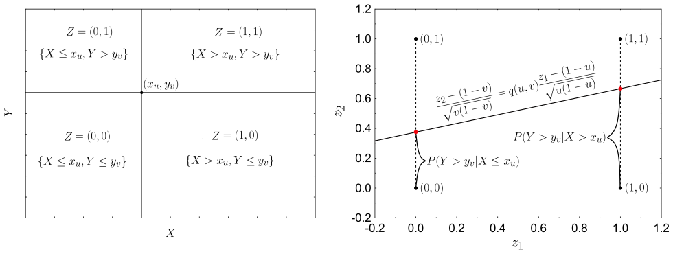
The authors introduce a new estimator of the quantile dependence function along with pertinent local acceptance regions. This combination yields an insightful visualization of the dependence structure and a rigorous test for independence between two random variables. The procedures are rank-based, admit finite-sample theory ensuring validity at any sample size, and the test is shown to be consistent and powerful across a wide range of alternatives.
What carries the argument
The quantile dependence function estimator, which measures dependence at different quantiles and is paired with local acceptance regions derived from its distribution under independence.
If this is right
- The method allows detection of local departures from independence in addition to global testing.
- The finite-sample theory ensures the procedures are valid without relying on large-sample approximations.
- The test ranks among the best in power for various dependence models.
- Visualization helps interpret the form of dependence in real data applications.
Where Pith is reading between the lines
- Such local visualization could extend to multivariate settings or time series dependence.
- The rank-based nature suggests robustness to outliers and applicability in nonparametric settings.
- Integration with machine learning pipelines might allow automated dependence screening in high dimensions.
Load-bearing premise
The quantile dependence function must adequately capture the relevant aspects of the dependence structure for the visualization and test to be meaningful.
What would settle it
A simulation study where the new test fails to rank among the most powerful across the claimed wide range of alternatives, or where the local acceptance regions do not correctly flag known dependence patterns at finite sample sizes.
Figures


read the original abstract
Identifying dependency between two random variables is a fundamental problem. The clear interpretability and ability of a procedure to provide information on the form of possible dependence is particularly important when exploring dependencies. In this paper, we introduce a novel method that employs a new estimator of the quantile dependence function and pertinent local acceptance regions. This leads to an insightful visualisation and a rigorous evaluation of the underlying dependence structure. We also propose a test of independence of two random variables, pertinent to this new estimator. Our procedures are based on ranks, and we derive a finite-sample theory that guarantees the inferential validity of our solutions at any given sample size. The procedures are simple to implement and computationally efficient. The large sample consistency of the proposed test is also proved. We show that, in terms of power, the new test is one of the best statistics for independence testing when considering a wide range of alternative models. Finally, we demonstrate the use of our approach to visualise dependence structure and to detect local departures from independence through analysing some real-world datasets.
Editorial analysis
A structured set of objections, weighed in public.
Referee Report
Summary. The paper introduces a rank-based estimator of the quantile dependence function together with explicitly constructed local acceptance regions. These are used both for visualization of dependence structure and for a test of independence between two random variables. The central claims are that the procedures possess exact finite-sample validity under the null of independence, that the test is large-sample consistent, and that it attains competitive power against a broad collection of alternatives.
Significance. A method that delivers exact finite-sample validity for both visualization and testing, while remaining computationally simple, would be a useful addition to the nonparametric independence-testing literature. The claimed power performance across alternatives, if substantiated, would further strengthen its practical value.
major comments (3)
- [§3] §3 (finite-sample theory): the derivation of the local acceptance regions from the exact null distribution of the rank-based estimator must be presented in full; without the explicit construction it is impossible to verify that the regions deliver exact (rather than approximate) validity at every finite n.
- [§4] §4 (power study): the statement that the test is 'one of the best' requires a tabulated comparison that includes the precise alternatives, sample sizes, and competing procedures; the current summary claim cannot be assessed without these details.
- [Theorem on large-sample consistency] Theorem on large-sample consistency: the proof must clarify the precise conditions on the quantile dependence function under which consistency holds; if the function is zero for certain forms of dependence, consistency would fail for those alternatives.
minor comments (2)
- [§2] The definition of the quantile dependence function and its estimator should appear before the construction of the acceptance regions to improve readability.
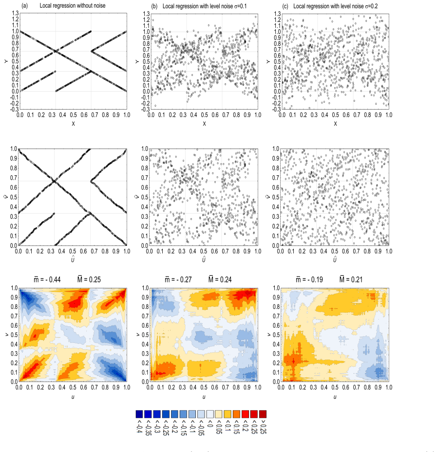
- [Figures 4-6] Figure captions for the real-data examples should explicitly state which acceptance regions are shown and at what nominal level.
Simulated Author's Rebuttal
We thank the referee for the careful reading and constructive comments on our manuscript. We address each major comment below, indicating the revisions we will make to strengthen the paper.
read point-by-point responses
-
Referee: §3 (finite-sample theory): the derivation of the local acceptance regions from the exact null distribution of the rank-based estimator must be presented in full; without the explicit construction it is impossible to verify that the regions deliver exact (rather than approximate) validity at every finite n.
Authors: We agree that the derivation in §3 requires a more explicit and complete presentation to demonstrate the exact finite-sample validity. We will expand this section with the full step-by-step construction of the local acceptance regions directly from the exact null distribution of the rank-based estimator. revision: yes
-
Referee: §4 (power study): the statement that the test is 'one of the best' requires a tabulated comparison that includes the precise alternatives, sample sizes, and competing procedures; the current summary claim cannot be assessed without these details.
Authors: We accept that the power comparison claim needs substantiation through a detailed table. In the revision we will add a comprehensive table in §4 that lists all alternatives considered, the sample sizes used, the competing procedures, and the resulting power values to allow direct assessment of the performance. revision: yes
-
Referee: Theorem on large-sample consistency: the proof must clarify the precise conditions on the quantile dependence function under which consistency holds; if the function is zero for certain forms of dependence, consistency would fail for those alternatives.
Authors: We will revise the statement and proof of the large-sample consistency theorem to explicitly delineate the conditions on the quantile dependence function that are required for consistency to hold. This will include a clear discussion of the class of alternatives for which the function is non-zero. revision: yes
Circularity Check
No significant circularity in derivation chain
full rationale
The paper introduces a novel rank-based estimator of the quantile dependence function along with explicitly derived finite-sample acceptance regions that guarantee exact validity under independence at any sample size. It separately proves large-sample consistency of the associated independence test and reports power comparisons across alternatives. These steps are presented as direct theoretical derivations rather than reductions to fitted parameters, self-definitions, or load-bearing self-citations. The central claims rest on independent mathematical results and do not collapse by construction to the inputs.
Axiom & Free-Parameter Ledger
axioms (1)
- standard math Finite-sample distributions of rank-based statistics can be derived exactly under independence.
Forward citations
Cited by 1 Pith paper
-
The post-hoc test for local dependence
A new testing procedure uses critical surfaces on the quantile dependence function to detect local dependence while preserving the global significance level.
Reference graph
Works this paper leans on
-
[1]
Journal of Machine Learning Research 6, 2075–2129
Kernel methods for measuring independence. Journal of Machine Learning Research 6, 2075–2129. H´ ajek, J.,ˇSid´ ak, Z.,
work page 2075
-
[2]
Dependence function for bivariate cdf's
Dependence function for bivariate cdf’s. arXiv:1405.2200v1 [stat.ME]. Ledwina, T.,
work page internal anchor Pith review Pith/arXiv arXiv
-
[3]
The sample sizes are: 88, 128, 230, 517 while d(n) are: 63, 63, 127, 255 accord- ingly
1 Supplementary Material A.1.The values of barriers in real data examples and their stability In this section, we reproduce on a larger scale the barriers appearing in our four real data examples. The sample sizes are: 88, 128, 230, 517 while d(n) are: 63, 63, 127, 255 accord- ingly. Throughout, we consider Πk,l, k, l = 1 , ...,10, as defined in Section 4...
work page 2020
-
[4]
Based on 100 000 MC repetitions. 4 A.2. Zhang’s BET framework. New interpretation and related comments To describe the nine patterns introduced by Zhang (2019) and exploited by Xiang et al. (2023) as well as Lee et al. (2023) we shall use the Walsh (1923) system of functions. We follow the description in Paley (1932). To define the needed elements, only t...
work page 2019
-
[5]
We have w0(s) ≡ 1, while w1(s) = r1(s), w 2(s) = r2(s) and w3(s) = r1(s)r2(s)
Next, recall the definition of the first four Walsh functions w0(s), w 1(s), w 2(s) and w3(s), s ∈ [0, 1). We have w0(s) ≡ 1, while w1(s) = r1(s), w 2(s) = r2(s) and w3(s) = r1(s)r2(s). The Walsh functions wj(s), j ≥ 1, take on only two values +1 and -1, on respective subintervals of [0,1) induced by the Rademacher system. Now, observe that the nine succe...
work page 2023
-
[6]
Since Walsh functions are orthonormal, (A.1) shows that Wi,j’s can also be seen as empirical correlation coefficients of relevant functions of observations. For readers accustomed to Zhang’s notation, we link our notation to the original ones: W1,1 = S(10,10), W 1,2 = S(10,01), W 1,3 = S(10,11), W 2,1 = S(01,10), W 2,2 = S(01,01), W 2,3 = S(01,11), W3,1 =...
work page 1999
-
[7]
that patterns are handy and useful in detecting and displaying some tendencies in allocation of pseudo-observations in [0, 1]2. On the other hand, it is also clear that in some situations the small set of templates is not rich enough and flexible. Zhang (2019), p. 1632, discusses some limitation of the approach in case of local dependency. Many other situ...
work page 2019
-
[8]
In the second row, related estimators ¯qn are depicted
In the first row, we present three scatter plots along with related dependence patterns indicated by Zhang’s procedure. In the second row, related estimators ¯qn are depicted. The third row shows pertinent dependence diagrams. A.3.1. Danish fire insurance data - a continuation As mentioned in Section 4.2, Gijbels and Sznajder (2013) have investigated thes...
work page 2013
-
[9]
A.3, although again our display seems to be easier readable
Their observations are fully consistent with outputs of ¯qn shown in our Fig. A.3, although again our display seems to be easier readable. The type of violation of the PQD structure appears to be relatively simple. It is mainly the gap in probability mass in the lower-left region accompanied by some tendency to grow towards the upper-right corner. These i...
work page 2013
-
[10]
A.3.2. Aircraft data We investigated the dependency between span (X) and speed (Y), on log scales, using the data set available at https://rdrr.io/cran/sm/. The graphic analysis of the dependence structure in this set can be found in Jones & Koch (2003). They relied on the local dependence function elaborated by Holland & Wang (1987) and Jones (1996). The...
work page 2003
-
[11]
These findings are consistent with our conclusions, although they give a much more raw picture of the situation. A.3.3. Temperature data Now we illustrate the use of our approach on the meteorological data set available at https://dane.imgw.pl/data/dane_pomiarowo_obserwacyjne/dane_meteorologiczne/dobowe/klimat/. We consider the average daily temperature i...
work page 2022
-
[12]
A.4. Full list of alternatives, empirical powers, and related comments We use the list of models proposed in Ćmiel & Ledwina (2020). It has been defined as follows. Simple Regression: SR1: Linear Y = 2 + X + ϵ, X ∼ U[0, 1], ϵ ∼ N(0, 1); SR2: Root Y = X 1/4 + ϵ, X ∼ U[0, 1], ϵ ∼ N(0, 0.25); SR3: Step Y = 1(X ≤ 0.5) + ϵ, X ∼ U[0, 1], ϵ ∼ N(0, 2); SR4: Logar...
work page 2020
-
[13]
Define X = X0, Y = ϵM Y0 + ϵA, ϵM ∼ N(0, 1), ϵ A ∼ N(0, 1)
+ ϵA, ϵ M ∼ N(0, 1), ϵ A ∼ N(0, 1); RE3: Reciprocal Y = ϵM X −1 + ϵA, ϵ M ∼ N(0, 1), ϵ A ∼ N(0, 1); RE4: Heavy tailed (X0, Y0) is bivariate Cauchy. Define X = X0, Y = ϵM Y0 + ϵA, ϵM ∼ N(0, 1), ϵ A ∼ N(0, 1). Classical Bivariate Models: BM1: Gaussian bivariate normal distribution with ρ = 0.3; BM2: Mixture I the mixture (0.1)(standard bivariate Gaussian) +...
work page 2020
-
[14]
Since this line is in fact the linear regression, the second part of Proposition 1 is proven
is equal to P (Y > y v|X > x u) − P (Y > y v|X ≤ xu). Since this line is in fact the linear regression, the second part of Proposition 1 is proven. The third part follows by properties of bivariate cdf and elementary transformations. □ A.5.2. Proof of Proposition 2 In formula (4) we have four terms, each of the structure kj(wj, zj)Cn(wj, zj), with adequat...
work page 1980
-
[15]
In this way, we also have an alternative simple proof of Proposition 1 in Ledwina and Wyłupek (2014). In view of the structure of ¯Cn(u, v) given byP4 j=1 kj(wj, zj)Cn(wj, zj), a similar argument 12 applies to ¯Cn(u, v) and thus concludes the proof of Proposition
work page 2014
-
[16]
This implies that sup (u,v)∈[c(n),1−c(n)]2 √n|A2(u, v)| = OP (2s(n)) = OP (d(n))
By Proposition 3.1 of Segers (2021), under our assumptions, √n| ˆCn(u, v) − C(u, v)| tends weakly, in the space ℓ∞([0, 1])2, to the Gaussian process (3.1) therein. This implies that sup (u,v)∈[c(n),1−c(n)]2 √n|A2(u, v)| = OP (2s(n)) = OP (d(n)). (A.3) When the null hypothesis is valid then A3(u, v) = 0 and we conclude that Tn ≤ OP (d(n)) ( A.4) under inde...
work page 2021
-
[17]
Since d(n)/√n → 0, by the assumption, (A.4) along with (A.6) imply the consistency under C
Hence 1 K(n) − κ(n) + 1 K(n)X k=κ(n) √n|A3|(k) ≥ √n a0 min{p0K(n), K(n) − κ(n) + 1} K(n) − κ(n) + 1 = O(√n) This yields Tn ≥ OP (√n) ( A.6) under the alternative C. Since d(n)/√n → 0, by the assumption, (A.4) along with (A.6) imply the consistency under C. □ A.6. Multivariate variants of q and ¯qn Consider a random vector X = ( X (1), ..., X(m)) with cont...
work page 1980
-
[18]
This is a counterpart of (5) in Section 3.1
o . This is a counterpart of (5) in Section 3.1. One can also check that ¯Cn is unbiased under independence, i.e. EH0 ¯Cn(t1, ..., tm) = mY k=1 tk. Under fixed n, the related expression for the variance of ¯Cn is quite complicated. Fortunately, by Theorem 3 form Deheuvels (1980), we have lim n→∞ VarH0Cn(t1, ..., tm)p n−1σ2(t1, ..., tm) = lim n→∞ VarH0 ¯Cn...
work page 1980
-
[19]
< m − 1, it holds that ¯Cn(t1, ..., tm) − mQ k=1 tk p n−1σ2(t1, ..., tm) D − − − → n→∞ N(0, 1), where D − →denotes convergence in distribution. In view of the above, we define the multivariate version of the quantile dependence function as q(t1, ..., tm) = C(t1, ..., tm) − mQ k=1 tk σ(t1, ..., tm) , 15 while its continuous multilinear estimator is defined...
work page 2014
-
[20]
Paley, R.E.A.C. (1932). A remarkable series of orthogonal functions (I). Proceedings of the London Mathematical Society 2, 241-264. R¨ uschendorf, L. (1980). Inequalities for the expectation of ∆-monotone functions. Zeitschrift f¨ ur Warscheinlichkeitstheorie und verwandte Gebiete54, 341-349. Schriever, B. (1987). An ordering for positive dependence. Anna...
work page 1932
discussion (0)
Sign in with ORCID, Apple, or X to comment. Anyone can read and Pith papers without signing in.