REVIEW 3 major objections 5 minor 22 references
From Instantaneous to Predictive Control: A More Intuitive and Tunable MPC Formulation for Robot Manipulators
T0 review · 3 major / 5 minor · reviewed 2026-08-12 · deepseek-v4-flash
Pith's one-line read A robot MPC whose stage cost penalizes deviation from a desired first-order response, preserving intuitive tuning while adding a prediction horizon.
desk verdict A practical MPC reparameterization that makes tuning more intuitive, but the headline time-constant property is only directly validated in simulation. read the letter →
The pith
A machine-rendered reading of the paper's core claim, the machinery that carries it, and where it could break.
The reading
What carries the argument
The load-bearing object is the stage cost $l_C(x_k,u_k)=\varepsilon(x_k,u_k)^\top W_s \varepsilon(x_k,u_k)+\mu u_k^\top W_r u_k$, where $\varepsilon(x,u)=\dot e(x,u)+K_e e(x)$ is the deviation from the desired first-order error response. This structure is the bridge between instantaneous and predictive control: it is algebraically equivalent to a particular choice of quadratic stage-cost matrices, but parameterized by $K_e$, whose entries are directly interpretable as task-error time constants $\alpha_i^{-1}$. A companion barrier-type inequality constraint uses the same first-order logic for constraints, so that constraints are activated with the same specified dynamics instead of requiring an infinitely fast reaction.
What would settle it
Run or simulate the proposed controller on a manipulator whose internal actuator dynamics have bandwidth only slightly above the chosen $\alpha_i$, and check whether the error still follows the specified exponential and whether changing the horizon leaves the transient unchanged; if the response becomes oscillatory or horizon-dependent, the central tuning claim fails.
Extended reading notes
Core claim
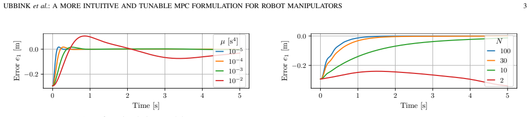
On the paper's own terms, the central discovery is that replacing the usual LQR-style stage cost with one that penalizes $\varepsilon = \dot e + K_e e$, the residual of a prescribed first-order response, lets the MPC inherit the tuning logic of instantaneous control: each diagonal entry $\alpha_i$ of $K_e$ directly sets the closed-loop time constant of the corresponding task error, and the response stays close to the specified exponential even when the horizon length changes. The weight $\mu$ on the control input retains only a regularization role; as long as it is small enough, the closed-loop behaviour is not sensitive to it. The paper further shows that inequality constraints can be imposed through the same mechanism, $\dot h(x,u)+K_h h(x)\ge \varepsilon_h$, so that constraints are approached with the same specified dynamics rather than infinitely fast. With a prediction horizon, the proposed controller anticipates upcoming constraints and thereby reduces tracking error and smooths accelerations compared to pure instantaneous control.
Load-bearing premise
The tuning claim presumes a speed gap in the real system: the desired time constants must be slow enough that the unmodeled actuator, sensor, and structural dynamics stay well out of the picture; otherwise the closed loop will not show the specified first-order response.
Editorial extensions
If this is right
- With constraints inactive, the closed-loop transient is independent of horizon length $N$, so changing the horizon for computational or constraint reasons does not force retuning.
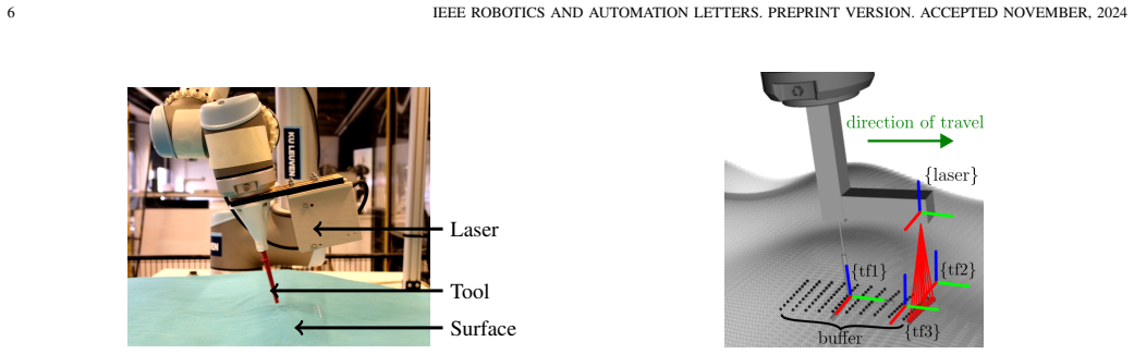
- Longer horizons improve constraint anticipation: in the surface-following experiment, longer horizons reduce surface-tracking RMSE, cut total task time by about 10%, and smooth joint accelerations.
- A working instantaneous controller can be upgraded to MPC incrementally by reusing its gains $K_e$ and adding a horizon.
- Tuning reduces to choosing the time constants and a small enough $\mu$, which also shrinks the search space for automated or learning-based tuning approaches.
- The formulation is not limited to robot manipulators; any system with task errors and a feedback model could use the same cost structure.
Reading between the lines
- The paper leaves implicit that the same stage cost gives MPC a per-task frequency-domain specification: choosing $\alpha_i$ is effectively choosing the closed-loop bandwidth of that error channel, which could later be connected to robustness margins under model uncertainty.
- A testable extension is to apply the formulation to systems with relative degree two using second-order desired dynamics along the horizon; the authors mention higher-order dynamics but do not pursue them.
- If the tuning property holds broadly, automated tuning methods could treat only the $\alpha_i$ values as decision variables, avoiding high-dimensional searches over arbitrary weight matrices.
- The control-barrier-function treatment of constraints suggests a route to safety guarantees under short horizons, but the paper does not provide formal stability or safety proofs; that is a natural next step.
Editorial analysis
A structured set of objections, weighed in public.
Referee Report
Summary. The paper proposes an MPC formulation for robot manipulators whose stage cost is l_C(x_k,u_k) = ε(x_k,u_k)^T W_s ε(x_k,u_k) + μ u_k^T W_r u_k, with ε(x,u) = \dot e(x,u) + K_e e(x). This makes the diagonal entries α_i of K_e interpretable as desired inverse time constants for the task errors. The paper first shows through a 3-DOF planar example that a conventional LQR-type stage cost leads to horizon- and weight-dependent closed-loop behavior, while the proposed cost produces approximately the same exponential error decay for N = 2, 10, 30, 100 in simulation. It then describes the equivalence of the proposed cost to a quadratic cost in (e, \dot e) with a block-structured weighting matrix (Eq. (14)), discusses CBF-type inequality constraints, and reports a UR10 surface-following experiment in which longer horizons reduce tracking RMSE, task time, and acceleration chattering. The paper is written from a practical perspective and makes its source code available.
Significance. The contribution is potentially valuable: if the tuning property is real, practitioners can specify first-order error dynamics through α_i^{-1} and still exploit a prediction horizon for constraint handling. The algebraic identity in Eq. (14) is a clean observation, and the paper makes its code available. The simulations are consistent with the claimed behavior, and the hardware results provide a plausible demonstration of the horizon benefit. The main weakness is that the central tuning claim—α_i sets the closed-loop time constant—is not directly validated on the hardware and is supported only by one idealized simulation with a single, unquantified separation margin.
major comments (3)
- [V-C, Fig. 10] The hardware experiment does not test the headline tuning property. It uses only α = 20 s^-1, does not vary α, and does not compare the measured surface-tracking error to the predicted first-order decay e0 exp(-α t). The RMSE and total-time results in Fig. 10 would be equally consistent with a closed-loop time constant that differs substantially from 0.05 s. Please add a direct experimental check of the α-to-time-constant map (e.g., a step response with two different α values and an overlay of the predicted envelope), or explicitly restrict the validation claim to horizon-length effects.
- [IV-C and Eq. (5)] The horizon-invariance and time-constant interpretation rely on a separation between the controller bandwidth α and the unmodeled actuator bandwidth α_internal. The paper reports a single ratio α/α_internal = 2/15 and states that the bandwidth was "selected to be significantly lower" without quantifying the margin needed for the 37%-time interpretation to hold. A sweep over α (or α_internal) would show how the closed-loop response degrades as the separation shrinks and would make the claimed tuning property reproducible.
- [IV-C and Eq. (3)] The property that the response is effectively independent of horizon length is demonstrated only by simulation, and no mechanism or analysis is offered for why the proposed stage cost should have this property, particularly since the related quadratic stage cost in Fig. 3 is strongly horizon dependent. Because no terminal cost is used and no stability proof is given, the central claim currently rests on a small set of examples. A brief analytical statement of the invariance condition, or at least an explicit statement of the empirical scope of the claim, would be needed to make the conclusion "regardless of horizon length" load-bearing.
minor comments (5)
- [VI] The conclusion contains a duplicated phrase: "ease of tuning and ease of tuning".
- [IV-C] Near Fig. 4a, state explicitly that the simulation uses α/α_internal = 2/15, so the reader does not have to infer the separation margin from the code or from the text.
- [IV-D] Explain why N ≥ 2 is necessary for first-order dynamics when the task has relative degree two; currently the reader must infer this from the discretized dynamics.
- [IV-A and II-B] Make explicit that the Q_B in Eq. (14) is not the diagonal Q_B = diag(I, λI) used in the motivating example, so Fig. 3 and Fig. 4a compare different stage-cost matrices.
- [V-C, Fig. 10] Report the number of experimental runs or add error bars; single runs make the RMSE and total-time differences across horizon lengths hard to assess.
Circularity Check
No circular derivation found; the proposed cost is an openly reparameterized quadratic objective, and the tuning claims are supported by simulation rather than fitted to data.
full rationale
The paper's central stage cost (Eqs. 12-13) is explicitly presented as a structured choice of quadratic weights, with the equivalence to the conventional objective stated openly in Eq. (14): 'by substituting (13) into (12) it is possible to show that this objective is equivalent to (6) when selecting QB = ...'. This is a transparent reparameterization, not a hidden reduction: ε is defined as the deviation from a first-order response, and the simulation in Fig. 4a demonstrates the resulting closed-loop behavior rather than being forced by a fitted parameter. No parameter is estimated from data and then renamed a prediction. The horizon-invariance and surface-following results are obtained from simulation and hardware experiments, not from the definition itself. Self-citations (Refs. [2], [20], [22]) supply the instantaneous-control vocabulary, the surface-following setup, and the solver, but none is load-bearing as a uniqueness theorem or as an unverified premise that replaces the paper's own argument. The admitted limitation in Section VI ('there is potential value in revisiting this approach from a more theoretical perspective') and the unquantified bandwidth-separation assumption in Section IV-C are correctness risks, not circularity. The score of 1 reflects the presence of self-citations and the lack of a formal theoretical guarantee, but the derivation chain is self-contained and non-circular.
Assumptions & free parameters
free parameters (4)
- Ke task-error gains (α_i) =
α=2 s^-1 (motivating example); α=20 s^-1 (hardware)
- Ws slack weights =
diag(1,1) s^2 m^-2 (example); w1..w5 = 1e2, 1e2, 1e2, 1e-2, 1e2 (hardware)
- Regularization μ =
1e-5 s^4 (example); 1e-6 s^4 (hardware)
- Wr input weight matrix =
diag(1 m^-2,1 rad^-2,1 rad^-2) (example); 1 rad^-2 (hardware)
assumptions (5)
- domain assumption The robot is an ideal acceleration-controlled system with control input u = \ddot q_cmd; in simulation, unmodeled actuator dynamics are first-order with α_internal = 15 s^-1.
- ad hoc to paper A finite-horizon MPC without terminal cost is stabilizing and achieves the desired closed-loop behavior.
- domain assumption The surface is locally well approximated by a quadratic model sθ, and the online least-squares estimate is accurate enough for control.
- domain assumption The nonlinear OCP is solved to a feasible near-optimal solution at 100 Hz by FATROP.
- domain assumption The controller bandwidth α is chosen below the bandwidth of unmodeled dynamics, so the model mismatch does not excite them.
Cite this review
Pith. "Pith review of From Instantaneous to Predictive Control: A More Intuitive and Tunable MPC Formulation for Robot Manipulators." pith.science (2026). https://pith.science/paper/RZ6KJHVT
@misc{pith2026241201597,
  author       = {Pith},
  title        = {Pith review of: From Instantaneous to Predictive Control: A More Intuitive and Tunable MPC Formulation for Robot Manipulators},
  year         = {2026},
  howpublished = {\url{https://pith.science/paper/RZ6KJHVT}},
  note         = {Machine review of arXiv:2412.01597}
}
read the original abstract
Model predictive control (MPC) has become increasingly popular for the control of robot manipulators due to its improved performance compared to instantaneous control approaches. However, tuning these controllers remains a considerable hurdle. To address this hurdle, we propose a practical MPC formulation which retains the more interpretable tuning parameters of the instantaneous control approach while enhancing the performance through a prediction horizon. The formulation is motivated at hand of a simple example, highlighting the practical tuning challenges associated with typical MPC approaches and showing how the proposed formulation alleviates these challenges. Furthermore, the formulation is validated on a surface-following task, illustrating its applicability to industrially relevant scenarios. Although the research is presented in the context of robot manipulator control, we anticipate that the formulation is more broadly applicable.
Figures


Figures from the paper (7 more)




Reference graph
Works this paper leans on
- [1]
-
[2]
E. Aertbeliën and J. De Schutter, “Etasl/etc: A constraint- based task specification language and robot controller using expression graphs,” in 2014 IEEE/RSJ Interna- tional Conference on Intelligent Robots and Systems , 2014
work page 2014
-
[3]
Sensor-based task-constrained motion planning using model predictive control,
M. Cefalo, E. Magrini, and G. Oriolo, “Sensor-based task-constrained motion planning using model predictive control,” in 12th IFAC Symposium on Robot Control , 2018
work page 2018
-
[4]
Model predictive interaction control for robotic manipulation tasks,
T. Gold, A. Völz, and K. Graichen, “Model predictive interaction control for robotic manipulation tasks,” IEEE Transactions on Robotics , 2023
work page 2023
-
[5]
Force Feedback Model-Predictive Control via Online Estimation,
A. Jordana, S. Kleff, J. Carpentier, N. Mansard, and L. Righetti, “Force Feedback Model-Predictive Control via Online Estimation,” in IEEE International Conference on Robotics and Automation , 2024
work page 2024
-
[6]
Frequency-aware model predictive control,
R. Grandia, F. Farshidian, A. Dosovitskiy, R. Ranftl, and M. Hutter, “Frequency-aware model predictive control,” IEEE Robotics and Automation Letters , 2019
work page 2019
-
[7]
Auto- mated tuning of nonlinear model predictive controller by reinforcement learning,
M. Mehndiratta, E. Camci, and E. Kayacan, “Auto- mated tuning of nonlinear model predictive controller by reinforcement learning,” in IEEE/RSJ International Conference on Intelligent Robots and Systems , 2018
work page 2018
-
[8]
Automatic tuning for data-driven model predictive control,
W. Edwards, G. Tang, G. Mamakoukas, T. Murphey, and K. Hauser, “Automatic tuning for data-driven model predictive control,” in 2021 IEEE International Conference on Robotics and Automation , 2021
work page 2021
Show all 22 references
-
[9]
Model predictive con- trol tuning by controller matching,
S. Di Cairano and A. Bemporad, “Model predictive con- trol tuning by controller matching,” IEEE Transactions on Automatic Control , 2010
2010
-
[10]
Model pre- dictive impedance control,
M. Bednarczyk, H. Omran, and B. Bayle, “Model pre- dictive impedance control,” in 2020 IEEE International Conference on Robotics and Automation , 2020
2020
-
[11]
Rawlings, D
J. Rawlings, D. Mayne, and M. Diehl, Model Predictive Control: Theory, Computation, and Design . Nob Hill Publishing, 2017
2017
-
[12]
Optimum settings for automatic controllers,
B. J. G. Ziegler and N. B. Nichols, “Optimum settings for automatic controllers,” Journal of Fluids Engineering, 1942
1942
-
[13]
On Weight-Prioritized Multitask Control of Humanoid Robots,
K. Bouyarmane and A. Kheddar, “On Weight-Prioritized Multitask Control of Humanoid Robots,” IEEE Transac- tions on Automatic Control , 2018
2018
-
[14]
Control bar- rier function based quadratic programs with application to adaptive cruise control,
A. D. Ames, J. W. Grizzle, and P. Tabuada, “Control bar- rier function based quadratic programs with application to adaptive cruise control,” in 53rd IEEE Conference on Decision and Control , 2014
2014
-
[15]
Safety-critical control for non-affine nonlinear systems with application on autonomous vehicle,
T. D. Son and Q. Nguyen, “Safety-critical control for non-affine nonlinear systems with application on autonomous vehicle,” in IEEE 58th Conference on Decision and Control , 2019
2019
-
[16]
Real-time mpc with control barrier functions for au- tonomous driving using safety enhanced collocation,
J. P. Allamaa, P. Patrinos, T. Ohtsuka, and T. D. Son, “Real-time mpc with control barrier functions for au- tonomous driving using safety enhanced collocation,” in IFAC Conference on Nonlinear Model Predictive Control, 2024
2024
-
[17]
Optimal nonlinear controllers for feedback linearizable systems,
R. Freeman and P. Kokotovic, “Optimal nonlinear controllers for feedback linearizable systems,” in Pro- ceedings of 1995 American Control Conference , 1995
1995
-
[18]
A receding horizon generalization of pointwise min-norm controllers,
J. Primbs, V . Nevistic, and J. Doyle, “A receding horizon generalization of pointwise min-norm controllers,” IEEE Transactions on Automatic Control , 2000
2000
-
[19]
Nonlinear model predictive control of robotic systems with control lyapunov functions,
R. Grandia, A. J. Taylor, A. W. Singletary, M. Hutter, and A. Ames, “Nonlinear model predictive control of robotic systems with control lyapunov functions,” in Robotics: Science and Systems , 2020
2020
-
[20]
Contactless surface following with accel- eration limits: Enhancing robot manipulator performance through model predictive control,
J. Ubbink, R. Viljoen, E. Aertbeliën, W. Decré, and J. D. Schutter, “Contactless surface following with accel- eration limits: Enhancing robot manipulator performance through model predictive control,” European Control Conference, 2024
2024
-
[21]
CasADi – A software framework for non- linear optimization and optimal control,
J. A. E. Andersson, J. Gillis, G. Horn, J. B. Rawlings, and M. Diehl, “CasADi – A software framework for non- linear optimization and optimal control,” Mathematical Programming Computation, 2019
2019
-
[22]
Fatrop: A fast constrained optimal control problem solver for robot trajectory optimization and control,
L. Vanroye, A. Sathya, J. De Schutter, and W. Decré, “Fatrop: A fast constrained optimal control problem solver for robot trajectory optimization and control,” IEEE/RSJ International Conference on Intelligent Robots and Systems, 2023
2023
Reviewed August 12, 2026 · model on record in the stance chip above.
Discussion (0). Continue with ORCID to comment.