REVIEW 3 major objections 4 minor 51 references
Efficient Multiple Temporal Network Kernel Density Estimation
T0 review · 3 major / 4 minor · reviewed 2026-08-10 · deepseek-v4-flash
Pith's one-line read The paper claims a per-edge range forest computes exact temporal network kernel-density values for all lixels in O(|E|(T_sp + L log(N/|E|))) time, with up to 6x speedup over prior work.
desk verdict Clever persistent-range-forest idea, but the endpoint-split decomposition is wrong for events on the query's own edge and Equation (4) has swapped entries, so the exactness claim fails as written. read the letter →
The pith
A machine-rendered reading of the paper's core claim, the machinery that carries it, and where it could break.
The reading
What carries the argument
The central object is the range forest: for each edge, a sequence of persistent range trees over events sorted by position, built one tree per timestamp, with unchanged subtrees shared across versions. DualDetect is the recursion that walks the two roots of the subtracted trees and returns the aggregation for the spatial range, and its claimed $O(\log n_e)$ cost rests on each level containing at most one partially covered node. DRFS makes the structure dynamic by splitting each edge by absolute position rather than by event count, extending the depth $H$ lazily, so a user can quantize the index and trade accuracy for memory and time. Lixel Sharing is a complementary mechanism that detects dominated edges and out-of-bandwidth edges to skip or bulk-update whole lixel sets via second-order differences.
What would settle it
Run RFS on a synthetic network with one edge $(v_c,v_d)$, a query lixel $q$, and an event $p$ sitting at a mid-edge junction whose shortest path from $q$ is shorter than both $d(q,v_c)+d(v_c,p)$ and $d(q,v_d)+d(v_d,p)$; compare RFS's KDE value with brute-force shortest-path summation. A mismatch would show the endpoint-decomposition assumption is violated.
Extended reading notes
Core claim
The paper's central claim is that temporal network KDE reduces to a range query on a per-edge persistent data structure. For each edge $(v_c,v_d)$, events are sorted by their distance from $v_c$ and inserted one by one into a range tree; because an insertion updates only $O(\log n_e)$ nodes, the sequence of trees forms a compact range forest. A query with time window $[T_l,T_r]$ subtracts tree $T_{l-1}$ from $T_r$, and a simultaneous recursion called DualDetect returns the aggregated vector for events whose positions along the edge satisfy the spatial bandwidth and the 'closer to $v_c$ than $v_d$' condition, in $O(\log n_e)$ per edge. The paper also claims the vector decomposition is exact for non-polynomial kernels: the exponential kernel factors as $e^{-d(q,v_c)/b_s}\sum e^{-d(v_c,p_i)/b_s}$, the cosine kernel splits into cosine and sine sums, and combined spatial-temporal kernels keep a constant-size aggregate vector. Lixel Sharing supplements the index by recognizing dominated edges where all lixels see the same aggregation, replacing per-lixel queries with second-order difference updates.
Load-bearing premise
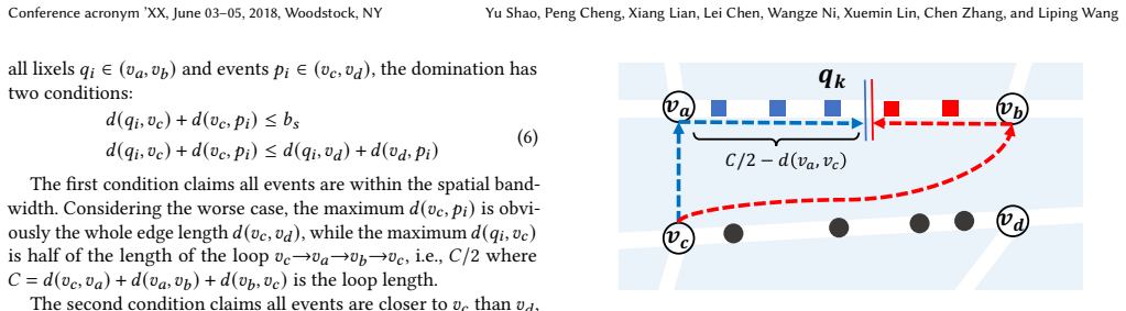
The method assumes each road edge is a straight line with exactly two endpoints, so every shortest path from a query lixel to an event on that edge goes through one of those two endpoints; if real edges have mid-edge junctions or bends, the per-edge decomposition and lixel counts change.
Editorial extensions
If this is right
- A query over any time window costs about the same as a query over all events, since the time subtraction is built into the tree pair; the reported processing time stays flat as the time-window size grows.
- Exponential and cosine kernels are computed exactly, so users are not restricted to polynomial kernels or polynomial approximations for network heatmaps.
- DRFS supports insertion of new events without rebuilding, and its depth $H$ controls a smooth accuracy/memory/time tradeoff, reaching over 99.9 percent accuracy at $H=10$ in the reported settings.
- Lixel Sharing removes dominated and out-of-bandwidth edges from the per-lixel loop, so the practical cost is governed by the residual edge set rather than all edges.
- On the reported real-road datasets, the speedups reach 6 times over ADA and 88.9 times over SPS for multiple online queries.
Reading between the lines
- The straight-line, two-endpoint edge model is the natural boundary of the exactness claim; on real roads with mid-edge junctions or significant shape points, the decomposition would likely need recursive subedge handling, which the paper does not discuss.
- Because the query-vector/aggregate-vector decomposition is agnostic to the kernel's analytic form, the same construction may extend to other separable spatial-temporal aggregation functions beyond the listed kernels; this is not claimed in the paper.
- The reported over-90-percent accuracy at $H=2$ suggests a practical tuning rule: begin with a shallow forest for coarse exploration, then deepen only regions of the heatmap that need detail; the paper does not implement spatially adaptive depth.
Editorial analysis
A structured set of objections, weighed in public.
Referee Report
Summary. The paper defines TN-KDE, a spatiotemporal kernel density estimation problem over road networks, and proposes the Range Forest Solution (RFS) as an exact method, together with a dynamic variant (DRFS), a Lixel Sharing (LS) optimization, and exact handling of non-polynomial kernel functions such as exponential and cosine. The algorithms organize events on each edge into persistent range trees indexed by time and answer spatial range queries by subtracting two tree states. The paper reports experimental speedups over ADA and SPS on four OpenStreetMap-derived datasets. The central claim is that RFS computes exact TN-KDE values for all lixels in O(|E|(T_sp + L log(N/|E|))) query time.
Significance. If the central claim were correct, the paper would offer a useful practical improvement for network KDE with temporal filtering, and the extension to exact non-polynomial kernels would be a genuine contribution. The paper is clearly written, the complexity analysis is transparent, and the experiments cover multiple datasets and parameter settings. However, the exactness claim is not supported: the endpoint-split decomposition on which RFS relies is invalid for events lying on the query lixel's own edge, and the central displayed formula in Equation (4) is internally inconsistent. Because the manuscript's headline contribution is exactness and speed based on that exactness, these are load-bearing defects rather than presentation issues.
major comments (3)
- [Section 3.2, Eq. (2), Eq. (4), Algorithm 1] The decomposition assumes that for an event p_i on edge e=(v_c,v_d), the shortest path from any query lixel q to p_i passes through exactly one of v_c or v_d. This is false when q itself lies on e. For a straight edge of length L with q at coordinate x and p_i at coordinate y, the network distance is |x-y|, but the endpoint formula gives min(x+y, (L-x)+(L-y)), which is generally larger. Algorithm 1 loops over all edges e for every lixel q without excluding the query's own edge, so for every lixel the contributions of events on its own edge are computed with an incorrect distance. Concretely, with L=100, b_s=100, q at 60m, p at 40m and the Triangular kernel, the true contribution is 1-20/100=0.8, while the endpoint formula gives 1-100/100=0.0. Thus the exactness claims of Lemma 4.3 and the experiments are not supported by the algorithm as presented.
- [Section 3.2, Eq. (4)] Equation (4) is printed incorrectly: the second and third entries of the query vector are swapped. The displayed dot product equals -sum d_i t_i + (b_s-d(q,v_c)) sum d_i - (b_t-t) sum t_i + (b_s-d(q,v_c))(b_t-t)|O|, while the preceding double-sum expands to (b_s-d(q,v_c))(b_t-t)|O| - (b_s-d(q,v_c)) sum t_i - (b_t-t) sum d_i + sum d_i t_i. The signs and coefficients do not match, so the formula cannot be used to implement the method. This is a load-bearing error because the query-vector/aggregated-vector product is the core operation in Algorithm 1 and in the derivation of RFS.
- [Section 5.2, Algorithm 2, quantization] The quantization description states that when the terminated node is partially covered, the returned value is a zero-vector. This means DRFS silently drops all events in that node rather than returning a partial aggregation. The paper acknowledges DRFS is approximate, but the accuracy results in Figure 20 are reported only as values over 90%; the zero-vector convention can produce large errors for small H. The effect should be evaluated explicitly, especially for events near the query lixel's own edge where the endpoint decomposition already fails.
minor comments (4)
- [Section 1, Keywords] The keyword 'Shorest Path' should be 'Shortest Path'.
- [Algorithm 2, Line 5] The return value 0 in the non-covered case should be a zero vector of the same length as A, not a scalar, to be consistent with the type of the aggregated vector.
- [Section 8.1] The assumption that each edge is a straight line is stated only in the experiments; it should be stated in the problem definition in Section 3, because the endpoint decomposition and the lixel-counting formulas depend on it.
- [Section 3.2 and Section 7] The paper should clarify whether the Lixel Sharing optimization applies only to the Triangular kernel; Section 7 presents non-polynomial kernels with a different product form, and the experimental comparison of RFS with LS against ADA should state which kernel and which version of RFS is used in each figure.
Circularity Check
No circularity: the TN-KDE derivation is self-contained; the endpoint-split issue is a correctness concern, not a circular-input concern.
full rationale
The paper's derivation chain is not circular. RFS is constructed directly from the TN-KDE definition in Definition 3.4 and the aggregation identities in Equations (3)-(4); the Q/A decomposition is a purely algebraic rearrangement of the kernel sum, and the exponential/cosine decompositions in Section 7 are trigonometric/exponential product identities. No parameter is fitted to the experimental output, and the DRFS accuracy numbers are measured against the static exact RFS rather than being enforced by construction. The paper's external reliance is on standard range-tree/persistence techniques (e.g., [18]) and on the ADA baseline [14], which is explicitly compared against rather than assumed as the target result. There are no load-bearing self-citations: the reference list contains no works by the present authors, and the 'state-of-the-art' ADA is cited as external prior work. Lemma 4.1's partial-coverage argument and Lemma 4.3's complexity bound are independent of the experiments. The reviewer's endpoint-split objection (events on the query's own edge) is a substantive correctness flaw in the inherited ADA decomposition, but it is an invalid-distance modeling error, not a case where a prediction is equivalent to its input; it therefore does not raise the circularity score under the stated rules.
Assumptions & free parameters
assumptions (3)
- domain assumption Shortest path distance is a metric, and the shortest path from any point on one edge to any point on another edge passes through exactly one of the target edge's endpoints.
- standard math A balanced range tree over events sorted by d(v_c,p_i) supports prefix aggregation queries in O(log n_e) with at most one partially covered node per level.
- domain assumption In the experiments, each road edge is a straight line, so d(v_c,p_i) and d(v_d,p_i) are linear in the position along the edge.
Cite this review
Pith. "Pith review of Efficient Multiple Temporal Network Kernel Density Estimation." pith.science (2026). https://pith.science/paper/KZOHXOAK
@misc{pith2026250107106,
  author       = {Pith},
  title        = {Pith review of: Efficient Multiple Temporal Network Kernel Density Estimation},
  year         = {2026},
  howpublished = {\url{https://pith.science/paper/KZOHXOAK}},
  note         = {Machine review of arXiv:2501.07106}
}
read the original abstract
Kernel density estimation (KDE) has become a popular method for visual analysis in various fields, such as financial risk forecasting, crime clustering, and traffic monitoring. KDE can identify high-density areas from discrete datasets. However, most existing works only consider planar distance and spatial data. In this paper, we introduce a new model, called TN-KDE, that applies KDE-based techniques to road networks with temporal data. Specifically, we introduce a novel solution, Range Forest Solution (RFS), which can efficiently compute KDE values on spatiotemporal road networks. To support the insertion operation, we present a dynamic version, called Dynamic Range Forest Solution (DRFS). We also propose an optimization called Lixel Sharing (LS) to share similar KDE values between two adjacent lixels. Furthermore, our solutions support many non-polynomial kernel functions and still report exact values. Experimental results show that our solutions achieve up to 6 times faster than the state-of-the-art method.
Figures


Figures from the paper (17 more)






Reference graph
Works this paper leans on
-
[1]
2023. [Online] ArcGIS. https://pro.arcgis.com/en/pro-app/latest/tool-reference/ spatial-analyst/kernel-density.htm
work page 2023
-
[2]
2023. [Online] QGIS. https://docs.qgis.org/3.22/en/docs/user_manual/ processing_algs/qgis/interpolation.html
work page 2023
-
[3]
James Abello, Frank Van Ham, and Neeraj Krishnan. 2006. Ask-graphview: A large scale graph visualization system. IEEE transactions on visualization and computer graphics 12, 5 (2006), 669–676. Publisher: IEEE
work page 2006
-
[4]
David Auber and Fabien Jourdan. 2005. Interactive refinement of multi-scale net- work clusterings. In Ninth International Conference on Information Visualisation (IV’05). IEEE, 703–709
work page 2005
-
[5]
William R Black. 1991. Highway accidents: a spatial and temporal analysis. Transportation Research Record 1318 (1991), 75–82
work page 1991
-
[6]
Giuseppe Borruso. 2005. Network density estimation: analysis of point patterns over a network. In International Conference on Computational Science and Its Applications. Springer, 126–132
work page 2005
-
[7]
Chris Brunsdon, Jonathan Corcoran, and Gary Higgs. 2007. Visualising space and time in crime patterns: A comparison of methods. Computers, environment and urban systems 31, 1 (2007), 52–75. Publisher: Elsevier
work page 2007
-
[8]
Michal Bíl, Richard Andrášik, and Zbyněk Janoška. 2013. Identification of haz- ardous road locations of traffic accidents by means of kernel density estimation and cluster significance evaluation. Accident Analysis & Prevention 55 (2013), 265–273. Publisher: Elsevier
work page 2013
Show all 51 references
-
[9]
Tsz Nam Chan, Reynold Cheng, and Man Lung Yiu. 2020. QUAD: Quadratic- bound-based kernel density visualization. InProceedings of the 2020 ACM SIGMOD International Conference on Management of Data . 35–50
2020
-
[10]
Tsz Nam Chan, Reynold Cheng, Man Lung Yiu, Shivansh Mittal, and others
-
[11]
Tsz Nam Chan, Pak Lon Ip, Leong Hou U, Byron Choi, and Jianliang Xu. 2021. SAFE: a share-and-aggregate bandwidth exploration framework for kernel den- sity visualization. Proceedings of the VLDB Endowment 15, 3 (2021), 513–526. Publisher: VLDB Endowment
2021
-
[12]
Tsz Nam Chan, Pak Lon Ip, Leong Hou U, Byron Choi, and Jianliang Xu. 2021. SWS: a complexity-optimized solution for spatial-temporal kernel density visual- ization. Proceedings of the VLDB Endowment 15, 4 (2021), 814–827. Publisher: VLDB Endowment
2021
-
[13]
Tsz Nam Chan, Pak Lon Ip, Leong Hou U, Weng Hou Tong, Shivansh Mittal, Ye Li, and Reynold Cheng. 2021. KDV-Explorer: A near real-time kernel density visualization system for spatial analysis. Proceedings of the VLDB Endowment 14, 12 (2021), 2655–2658. Publisher: VLDB Endowment
2021
-
[14]
Tsz Nam Chan, Zhe Li, Leong Hou U, Jianliang Xu, and Reynold Cheng. 2021. Fast augmentation algorithms for network kernel density visualization. Proceedings of the VLDB Endowment 14, 9 (2021), 1503–1516. Publisher: VLDB Endowment
2021
-
[15]
Tsz Nam Chan, Man Lung Yiu, and Hou U Leong. 2019. KARL: Fast kernel aggre- gation queries. In 2019 IEEE 35th International Conference on Data Engineering (ICDE). IEEE, 542–553
2019
-
[16]
Tao Cheng, James Haworth, and Jiaqiu Wang. 2012. Spatio-temporal autocorrela- tion of road network data. Journal of Geographical Systems 14 (2012), 389–413
2012
-
[17]
Nello Cristianini, Colin Campbell, and John Shawe-Taylor. 1998. Dynamically adapting kernels in support vector machines. Advances in neural information processing systems 11 (1998)
1998
-
[18]
Mark De Berg. 2000. Computational geometry: algorithms and applications . Springer Science & Business Media
2000
-
[19]
Matteo De Felice, Marcello Petitta, and Paolo M Ruti. 2015. Short-term predictabil- ity of photovoltaic production over Italy. Renewable Energy 80 (2015), 197–204. Publisher: Elsevier
2015
-
[20]
Diebold, Todd A
Francis X. Diebold, Todd A. Gunther, and Anthony S. Tay. 1998. Evaluating Density Forecasts with Applications to Financial Risk Management. International Economic Review 39, 4 (1998), 863–883. http://www.jstor.org/stable/2527342 Publisher: [Economics Department of the Universi...
1998
-
[21]
Francis X Diebold, Jinyong Hahn, and Anthony S Tay. 1999. Multivariate density forecast evaluation and calibration in financial risk management: high-frequency returns on foreign exchange. Review of Economics and Statistics 81, 4 (1999), 661–
1999
-
[22]
Jianqing Fan and James S Marron. 1994. Fast implementations of nonparametric curve estimators. Journal of computational and graphical statistics 3, 1 (1994), 35–56. Publisher: Taylor & Francis
1994
-
[23]
Paulo Figueiras, Zala Herga, Guilherme Guerreiro, António Rosa, Ruben Costa, and Ricardo Jardim-Gonçalves. 2018. Real-time monitoring of road traffic us- ing data stream mining. In 2018 IEEE International Conference on Engineering, Technology and Innovation (ICE/ITMC). IEEE, 1–8
2018
-
[24]
François Fleuret, Hichem Sahbi, and others. 2003. Scale-invariance of support vector machines based on the triangular kernel. In 3rd International Workshop on Statistical and Computational Theories of Vision . 1–13
2003
-
[25]
Edward Gan and Peter Bailis. 2017. Scalable kernel density classification via threshold-based pruning. In Proceedings of the 2017 ACM International Conference on Management of Data . 945–959
2017
-
[26]
Wei Gong, Dawen Yang, Hoshin V Gupta, and Grey Nearing. 2014. Estimating information entropy for hydrological data: One-dimensional case.Water Resources Research 50, 6 (2014), 5003–5018. Publisher: Wiley Online Library
2014
-
[27]
Artur Gramacki. 2018. Nonparametric kernel density estimation and its computa- tional aspects. Vol. 37. Springer
2018
-
[28]
Alexander G Gray and Andrew W Moore. 2003. Nonparametric density es- timation: Toward computational tractability. In Proceedings of the 2003 SIAM International Conference on Data Mining . SIAM, 203–211
2003
-
[29]
Timothy Hart and Paul Zandbergen. 2014. Kernel density estimation and hotspot mapping: Examining the influence of interpolation method, grid cell size, and bandwidth on crime forecasting. Policing: An International Journal of Police Strategies & Management 37, 2 (2014), 305–32...
2014
-
[30]
Andrew Harvey and Vitaliy Oryshchenko. 2012. Kernel density estimation for time series data. International journal of forecasting 28, 1 (2012), 3–14. Publisher: Elsevier
2012
-
[31]
Alexander Hinneburg and Hans-Henning Gabriel. 2007. Denclue 2.0: Fast cluster- ing based on kernel density estimation. In International symposium on intelligent data analysis. Springer, 70–80
2007
-
[32]
Nick Koudas, Beng Chin Ooi, Kian-Lee Tan, and Rui Zhang. 2004. Approximate NN queries on streams with guaranteed error/performance bounds. InProceedings of the Thirtieth international conference on Very large data bases-Volume 30 . 804– 815
2004
-
[33]
Matej Kristan, Aleš Leonardis, and Danijel Skočaj. 2011. Multivariate online kernel density estimation with Gaussian kernels. Pattern Recognition 44, 10-11 (2011), 2630–2642. Publisher: Elsevier
2011
-
[34]
Chenhui Li, George Baciu, and Yu Han. 2014. Interactive visualization of high density streaming points with heat-map. In 2014 International Conference on Smart Computing. IEEE, 145–149
2014
-
[35]
Tianyi Li, Lu Chen, Christian S Jensen, and Torben Bach Pedersen. 2021. TRACE: Real-time compression of streaming trajectories in road networks. Proceedings of the VLDB Endowment 14, 7 (2021), 1175–1187
2021
-
[36]
Zhicheng Liu, Biye Jiang, and Jeffrey Heer. 2013. imMens: Real-time visual querying of big data. In Computer Graphics Forum, Vol. 32. Wiley Online Library, 421–430. Issue: 3pt4
2013
-
[37]
Kyriakos Mouratidis, Man Lung Yiu, Dimitris Papadias, and Nikos Mamoulis
-
[38]
Tomoki Nakaya and Keiji Yano. 2010. Visualising crime clusters in a space-time cube: An exploratory data-analysis approach using space-time kernel density estimation and scan statistics. Transactions in GIS 14, 3 (2010), 223–239. Publisher: Wiley Online Library
2010
-
[39]
Roberto Patuelli, Aura Reggiani, Sean P Gorman, Peter Nijkamp, and Franz-Josef Bade. 2007. Network analysis of commuting flows: A comparative static approach to German data. Networks and Spatial Economics 7 (2007), 315–331
2007
-
[40]
Charlotte Plug, Jianhong Cecilia Xia, and Craig Caulfield. 2011. Spatial and tem- poral visualisation techniques for crash analysis. Accident Analysis & Prevention 43, 6 (2011), 1937–1946. Publisher: Elsevier
2011
-
[41]
Suman Rakshit, Adrian Baddeley, and Gopalan Nair. 2019. Efficient code for second order analysis of events on a linear network.Journal of Statistical Software 90 (2019), 1–37
2019
-
[42]
Benjamin Romano and Zhe Jiang. 2017. Visualizing traffic accident hotspots based on spatial-temporal network kernel density estimation. In Proceedings of the 25th ACM SIGSPATIAL International Conference on Advances in Geographic Information Systems. 1–4
2017
-
[43]
M Samiuddin and GM El-Sayyad. 1990. On nonparametric kernel density esti- mates. Biometrika 77, 4 (1990), 865–874. Publisher: Oxford University Press
1990
-
[44]
I Sasikala, M Ganesan, and A John. 2014. Uncertain data prediction on dynamic road network. In International Conference on Information Communication and Embedded Systems (ICICES2014). IEEE, 1–4
2014
-
[45]
Bernhard Scholkopf, Kah-Kay Sung, Christopher JC Burges, Federico Girosi, Partha Niyogi, Tomaso Poggio, and Vladimir Vapnik. 1997. Comparing support vector machines with Gaussian kernels to radial basis function classifiers. IEEE transactions on Signal Processing 45, 11 (1997)...
1997
-
[46]
Bernhard W Silverman. 1982. Algorithm AS 176: Kernel density estimation using the fast Fourier transform. Journal of the Royal Statistical Society. Series C (Applied Statistics) 31, 1 (1982), 93–99. Publisher: JSTOR
1982
-
[47]
Bernard W Silverman. 2018. Density estimation for statistics and data analysis . Routledge
2018
-
[48]
Zhixiao Xie and Jun Yan. 2008. Kernel density estimation of traffic accidents in a network space. Computers, environment and urban systems 32, 5 (2008), 396–406. Publisher: Elsevier
2008
-
[673]
Publisher: MIT Press 238 Main St., Suite 500, Cambridge, MA 02142-1046, USA journals
-
[2006]
Continuous nearest neighbor monitoring in road networks. (2006)
2006
-
[2020]
IEEE Transactions on Knowledge and Data Engineering (2020)
Efficient algorithms for kernel aggregation queries. IEEE Transactions on Knowledge and Data Engineering (2020). Publisher: IEEE
2020
Reviewed August 10, 2026 · model on record in the stance chip above.
Discussion (0). Continue with ORCID to comment.