REVIEW 3 major objections 4 minor 30 references
Magnetically assisted vorticity production in decaying acoustic turbulence
T0 review · 3 major / 4 minor · reviewed 2026-08-09 · deepseek-v4-flash
Pith's one-line read This paper argues that uniform magnetic fields convert a fraction of acoustic-turbulence energy into vortical motion, with vorticity growing quadratically in the field and linearly in sound amplitude, and that acoustic turbulence has a…
desk verdict A clean 1D derivation plus open 1024^3 MHD runs give a plausible new scaling for magnetically assisted vorticity conversion, but the broad universality claims outrun the evidence: the shock contribution is never separated and the fitted factor 71 is unexplained. read the letter →
The pith
A machine-rendered reading of the paper's core claim, the machinery that carries it, and where it could break.
The reading
What carries the argument
The load-bearing object is the linearized conversion identity $w_z=(v_{Ax}v_{Ay}/c_s^2)u_0 k$ for a standing sound wave in a uniform, non-aligned magnetic field. It comes from taking two time derivatives of the vorticity equation: the sound wave bends the initially uniform field, the resulting current density has a spatial gradient, and the curl of the Lorentz force accelerates a transverse velocity component whose derivative is the vorticity. In the turbulent three-dimensional setting, the same physics is expressed as $\mathrm{Ma}_V\propto \mathrm{Ma}_{M0}^2\,\mathrm{Ma}_A$ with empirical prefactor 0.67, and the acoustic Kolmogorov constant $C_K\approx6$ serves as the second quantitative signature distinguishing acoustic from vortical cascades.
What would settle it
Measure vorticity production for a standing sound wave in a uniform magnetic field at a Mach number low enough that shocks never form, and test whether $w_z$ follows $(v_{Ax}v_{Ay}/c_s^2)u_0 k$ when $u_0$ and $B_0$ are each varied by a factor of two; a clean alternative is to disable the induction term, as in the paper's run with induction off, and confirm that the quadratic term disappears while only the linear direct Lorentz-force channel remains.
Extended reading notes
Core claim
The paper's central discovery is that the Lorentz force can generate vorticity from a purely acoustic velocity field even when the magnetic field is initially uniform and force-free. The mechanism is quantified by $w_z=(v_{Ax}v_{Ay}/c_s^2)u_0 k$, obtained from the linearized induction and momentum equations for a standing sound wave in a uniform diagonal field, and confirmed numerically in one and three dimensions. In the three-dimensional turbulent runs with an imposed uniform field, the vortical Mach number follows $\mathrm{Ma}_V \approx 0.67\,\mathrm{Ma}_{M0}^2\,\mathrm{Ma}_A$; for a turbulent seed field, the same scaling holds with an effective field amplification factor of roughly 71. A separate, weaker channel produces vorticity linearly in the field strength when the field is not force-free, with the vortical kinetic spectrum approaching equipartition with the magnetic spectrum at high wavenumbers. The paper also establishes that acoustic turbulence obeys Kolmogorov phenomenology with a constant spectral flux and a nondimensional prefactor $C_K\approx6$, reduced to about 2\textendash 3 when magnetic fields are present.
Load-bearing premise
The derivation assumes constant density, a pure standing sound wave, and a uniform diagonal magnetic field, neglecting nonlinear feedback, Alfvén dynamics, and shock formation; the three-dimensional extension relies on those effects being subdominant, but in the strongest-field runs shocks are present and their vorticity contribution is not separated from the Lorentz-force contribution.
Editorial extensions
If this is right
- Phase-transition acoustic turbulence in the early universe, in the presence of a seed magnetic field, should develop a vortical component with amplitude controlled by the square of the magnetic field and the linear acoustic amplitude.
- The acoustic Kolmogorov constant near 6 means acoustic-dominated flows carry more energy at a given dissipation rate than vortical flows, so decay timescales inferred using the standard $1.6$ value would be too short.
- A turbulent magnetic field of strength $\mathrm{Ma}_{M1}\approx0.005$ acts like a uniform field roughly 71 times stronger, so very weak random seed fields can open the conversion channel.
- The direct Lorentz-force channel from a non-force-free field remains linear in field strength, so observations could distinguish the two mechanisms by measuring how vortical energy scales with field strength.
Reading between the lines
- The effective amplification factor of about 71 for turbulent fields suggests the early-universe seed fields needed to generate dynamically interesting vorticity could be substantially weaker than the strength implied by a naive uniform-field estimate.
- Shocks visible in the strongest field run ($\mathrm{Ma}_{M0}=1$) are a competing vorticity source; if they dominate, the quadratic scaling would saturate or steepen at higher Mach numbers, so the cleanest test of the conversion mechanism is at lower Mach with the same field strength.
- The same mechanism should operate in any barotropic or isothermal flow where acoustic waves cross a magnetic field, which makes the scaling testable in laboratory experiments with transducers and imposed magnetic fields, not just cosmological simulations.
Editorial analysis
A structured set of objections, weighed in public.
Referee Report
Summary. The paper investigates decaying acoustic (irrotational) subsonic turbulence with and without magnetic fields using 1024^3 simulations. The central claims are threefold: (i) the acoustic kinetic energy cascade exhibits Kolmogorov scaling with a constant spectral flux and a nondimensional prefactor larger than the standard Kolmogorov constant; (ii) a magnetic field, even if initially uniform, converts a fraction of acoustic energy into vortical energy with amplitude scaling wz = (vAx vAy/cs^2) u0 k, as derived from a 1D model in Section 3.6.1 and asserted to be validated by 3D runs in Figure 8; and (iii) turbulent magnetic fields produce the same conversion when rescaled by an empirical factor of 71. The authors discuss implications for vorticity generation in cosmological phase transitions.
Significance. If fully established, the magnetically assisted conversion mechanism would provide a concrete route from acoustic to vortical turbulence in the early Universe, and a robust Kolmogorov prefactor for acoustic turbulence would be a new quantitative benchmark. Strengths of the paper include a transparent and elegant 1D analytic derivation of Eq. (14), a systematic set of numerical experiments with resolutions up to 1024^3, and the public release of code and reduced data, which makes the results reproducible. However, the 3D validation of the central scaling relies on fitted prefactors (0.67 and 71), excludes several runs post hoc, and does not isolate the vorticity produced by the Lorentz force from that generated by shocks, which the paper itself shows to be present. The Kolmogorov prefactor claim is also internally inconsistent across sections. The significance is therefore conditional on resolving these issues.
major comments (3)
- [Section 3.6.2, Figure 8] The validation of the 1D scaling relies on the empirical relation MaV ≈ 0.67 MaM0^2 MaA, where 0.67 is not predicted by Eq. (14), and the runs with 0.02 ≤ MaM1 ≤ 0.2 (Runs I–L) are excluded with the only stated justification being that the magnetic field is weak and the acoustic turbulence strong. This exclusion removes the regime in which the predicted quadratic dependence is most likely to be tested, and no quantitative criterion is provided. The factor 71 used to map turbulent field strength to an equivalent uniform-field strength is likewise empirical; it is an additional free parameter with no derivation or independent confirmation. Please state the exclusion rule, report the fit including all runs, and estimate the uncertainty in the prefactor.
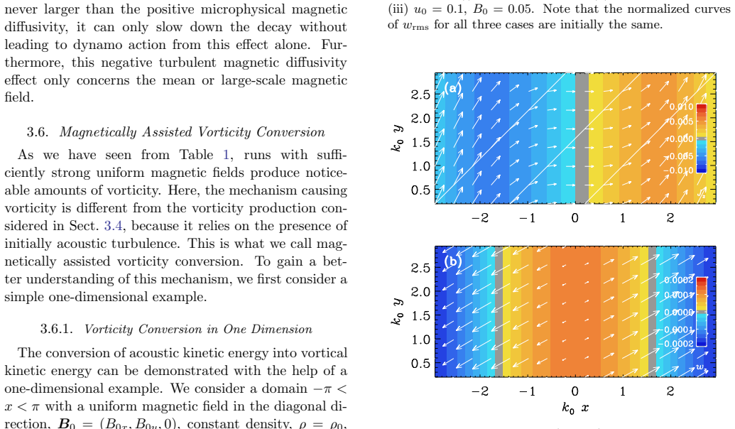
- [Section 3.6.2 and Figure 9; Equations (5)–(6)] Run N, which is one of the primary upholders of the scaling in Figure 8, shows shocks extending over major parts of the domain, and the text explicitly states that the shocks are especially clear in the vorticity maps. The 1D model in Section 3.6.1 assumes constant density, a uniform diagonal field, and no nonlinear steepening, so it excludes exactly the density variations that generate shocks. Equations (5) and (6) show that viscous vorticity production via G_i = 2S_ij ∂_j ln ρ occurs even without magnetic fields, and the Lorentz force at shock-generated current layers can also contribute. The paper does not separate shock-produced vorticity from magnetically assisted conversion, so the measured MaV in the 3D runs may include a substantial hydrodynamic contribution that is not described by Eq. (14). I request a control run with the same initial acoustic field and no magnetic field, or a budget of the individual production terms, to support the attribution.
- [Abstract, Section 3.3, and Section 4] The abstract and conclusions claim that acoustic turbulence follows ordinary Kolmogorov phenomenology with a constant spectral flux and a prefactor CK ≈ 6, larger than the vortical value of 1.6. However, Section 3.3 reports CA ≈ 8 for Run B and states that this 'suggest[s] that the standard Kolmogorov phenomenology may not be applicable', and the value CK ≈ 6 appears only in the conclusions without reconciliation. No error bars are given for either value. Because the Kolmogorov constant is a central quantitative result, the manuscript must either consistently present these measurements or explicitly reinterpret them as a test of the Kolmogorov hypothesis, and should report uncertainties.
minor comments (4)
- [Section 2.4, Equations (10)–(11)] The text notes that εK ≠ εV + εA due to mixed terms, but the definitions of εV and εA include only the diagonal contributions k^2EV and k^2EA. Please state explicitly whether the mixed terms were included or neglected in the reported Kolmogorov prefactors.
- [Table 1] The column labeled MaK is not defined in Section 2.4, where MaV and MaA are introduced. Please define MaK or rename the column to MaV if that is the intended quantity.
- [Figure 1 caption] The caption refers to 'Runs V', but Table 1 contains no Run V. Presumably this is a typo for Run A or Run B; please correct it.
- [Section 3.3, Figure 2 and 3] The insets are mentioned in the text but the axes and labels are not legible in the provided figures. Please ensure all inset panels include axis labels or a clear explanation in the caption.
Circularity Check
No significant circularity: Eq. (14) is derived from the MHD equations, and the 3D scaling is an empirical fit with a physical confounding from shocks, not a self-referential construction.
full rationale
The central claim, that a uniform magnetic field converts acoustic into vortical energy with wz = (vAx vAy/cs^2) u0 k, is obtained in Sec. 3.6.1 by an explicit calculation: the paper writes the uncurled induction equation and momentum equation, takes two time derivatives of the vorticity, substitutes Jz = -Az'', and uses the sound-wave dispersion relation omega = cs k. The result is not assumed as an input; it follows from the stated equations for a standing sound wave with constant density and uniform diagonal field. The later 3D plots in Sec. 3.6.2 fit a coefficient (0.67) and an empirical conversion factor (~71) for turbulent fields, but these are amplitudes and conversion factors, not the quadratic-in-B, linear-in-u functional form. The functional form itself is predicted independently. The Kolmogorov prefactor CK ~ 6 is read off a compensated-spectrum plateau; it is a measurement, not a fitted parameter relabeled as a prediction. Self-citations to Mee & Brandenburg (2006) and Kahniashvili et al. (2012) provide standard formulas and context, but they are not load-bearing for the new derivation. One genuine limitation, which the manuscript itself acknowledges in Fig. 9, is that Run N shows shocks 'extending over major parts of the domain' and vorticity maps that make the shocks 'especially clear'; isothermal shocks can produce vorticity through the viscous term nu x G in Eq. (5), and the paper does not separate this hydrodynamic shock-generated vorticity from the magnetically assisted contribution. That is an experimental/decomposition weakness that affects how strongly the 3D runs confirm the mechanism, but it is not circularity by construction. No step in the derivation reduces to its own output or to a fitted quantity presented as a first-principles prediction.
Assumptions & free parameters
free parameters (3)
- Kolmogorov prefactor CK for acoustic turbulence =
approximately 6 (Run B)
- Conversion prefactor 0.67 =
0.67
- Turbulent-to-uniform field mapping factor 71 =
approximately 71
assumptions (4)
- domain assumption Isothermal equation of state p = rho c_s^2
- domain assumption Helmholtz decomposition of the velocity field into vortical (EV) and acoustic (EA) parts, with EA approximately Elnrho
- standard math Kolmogorov dimensional cascade: E(k) proportional to epsilon^(2/3) k^(-5/3) with constant energy flux
- ad hoc to paper 1D model assumptions: uniform density, ux = u0 sin kx, uniform diagonal B0, neglect of nonlinear back-reaction
Cite this review
Pith. "Pith review of Magnetically assisted vorticity production in decaying acoustic turbulence." pith.science (2026). https://pith.science/paper/ABN2TBK7
@misc{pith2026250118525,
  author       = {Pith},
  title        = {Pith review of: Magnetically assisted vorticity production in decaying acoustic turbulence},
  year         = {2026},
  howpublished = {\url{https://pith.science/paper/ABN2TBK7}},
  note         = {Machine review of arXiv:2501.18525}
}
read the original abstract
We study vorticity production in isothermal, subsonic, acoustic (nonvortical), and decaying turbulence due to the presence of magnetic fields. Using three-dimensional numerical simulations, we find that the resulting kinetic energy cascade follows the ordinary Kolmogorov phenomenology involving a constant spectral energy flux. The nondimensional prefactor for acoustic turbulence is larger than the standard Kolmogorov constant due to the inefficient dissipation of kinetic energy. We also find that the Lorentz force can drive vortical motions even when the initial field is uniform, by converting a fraction of the acoustic energy into vortical energy. This conversion is shown to be quadratic in the magnetic field strength and linear in the acoustic flow speed. By contrast, the direct production of vortical motions by a non-force-free magnetic field is linear in the field strength. Our results suggest that magnetic fields play a crucial role in vorticity production in cosmological flows, particularly in scenarios where significant acoustic turbulence is prevalent. We also discuss the implications of our findings for the early Universe, where magnetic fields may convert acoustic turbulence generated during cosmological phase transitions into vortical turbulence.
Figures


Figures from the paper (6 more)



Reference graph
Works this paper leans on
-
[1]
Taking control of compressible modes: bulk viscosity and the turbulent dynamo
Bhattacharjee, A. 2023, arXiv e-prints, arXiv:2312.03984 , doi: 10.48550/arXiv.2312.03984
work page Pith review arXiv doi:10.48550/arxiv.2312.03984 2023
-
[2]
2023, MNRAS, 518, 6367, doi: 10.1093/mnras/stac3555
Brandenburg, A., Rogachevskii, I., & Schober, J. 2023, MNRAS, 518, 6367, doi: 10.1093/mnras/stac3555
-
[3]
2005, ThCFD, 19, 127, doi: 10.1007/s00162-004-0157-x Del Sordo, F., & Brandenburg, A
Cho, J., & Lazarian, A. 2005, ThCFD, 19, 127, doi: 10.1007/s00162-004-0157-x Del Sordo, F., & Brandenburg, A. 2011, A&A, 528, A145, doi: 10.1051/0004-6361/201015661 Elias-L´ opez, A., Del Sordo, F., & Vigan` o, D. 2023, A&A, 677, A46, doi: 10.1051/0004-6361/202346696 —. 2024, A&A, 690, A77, doi: 10.1051/0004-6361/202450398
-
[4]
1974, PhLA, 47, 419, doi: 10.1016/0375-9601(74)90155-8 —
Elsasser, K., & Schamel, H. 1974, PhLA, 47, 419, doi: 10.1016/0375-9601(74)90155-8 —. 1976, ZPhyB, 23, 89, doi: 10.1007/BF01322265
-
[5]
1994, PhFl, 6, 1411, doi: 10.1063/1.868255
Falkovich, G. 1994, PhFl, 6, 1411, doi: 10.1063/1.868255
doi:10.1063/1.868255 1994
-
[6]
1996, PhRvE, 54, 4431, doi: 10.1103/PhysRevE.54.4431
Falkovich, G., & Meyer, M. 1996, PhRvE, 54, 4431, doi: 10.1103/PhysRevE.54.4431
-
[7]
2011, PhRvL, 107, 114504, doi: 10.1103/PhysRevLett.107.114504
Federrath, C., Chabrier, G., Schober, J., et al. 2011, PhRvL, 107, 114504, doi: 10.1103/PhysRevLett.107.114504
-
[8]
Federrath, C., Schober, J., Bovino, S., & Schleicher, D. R. G. 2014, ApJL, 797, L19, doi: 10.1088/2041-8205/797/2/L19
Show all 30 references
-
[9]
1995, Turbulence
Frisch, U. 1995, Turbulence. The legacy of A.N. Kolmogorov (Cambridge University Press), doi: 10.1017/CBO9781139170666
1995 doi
-
[10]
2011, PhRvL, 107, 134501, doi: 10.1103/PhysRevLett.107.134501
Galtier, S., & Banerjee, S. 2011, PhRvL, 107, 134501, doi: 10.1103/PhysRevLett.107.134501
2011 doi
-
[11]
E., Brandenburg, A., & Dobler, W
Haugen, N. E., Brandenburg, A., & Dobler, W. 2004, PhRvE, 70, 016308, doi: 10.1103/PhysRevE.70.016308
2004 doi
-
[12]
J., Rummukainen, K., & Weir, D
Hindmarsh, M., Huber, S. J., Rummukainen, K., & Weir, D. J. 2015, PhRvD, 92, 123009, doi: 10.1103/PhysRevD.92.123009
2015 doi
-
[13]
S., & Madnia, C
Jahanbakhshi, R., Vaghefi, N. S., & Madnia, C. K. 2015, PhFl, 27, 105105, doi: 10.1063/1.4933250
2015 doi
-
[14]
B., & Petviashvili, V
Kadomtsev, B. B., & Petviashvili, V. I. 1973, SPhD, 18, 115
1973
-
[15]
Kahniashvili, T., Brandenburg, A., Campanelli, L., Ratra, B., & Tevzadze, A. G. 2012, PhRvD, 86, 103005, doi: 10.1103/PhysRevD.86.103005
2012 doi
-
[16]
2003, PhFl, 15, L21, doi: 10.1063/1.1539855
Uno, A. 2003, PhFl, 15, L21, doi: 10.1063/1.1539855
2003 doi
-
[17]
Kazantsev, A. P. 1968, JETP, 26, 1031
1968
-
[18]
P., Ruzmaikin, A
Kazantsev, A. P., Ruzmaikin, A. A., & Sokolov, D. D. 1985, ZhETF, 61, 285
1985
-
[19]
A., & Kuznetsov, E
Kochurin, E. A., & Kuznetsov, E. A. 2022, JETPL, 116, 863, doi: 10.1134/S0021364022602494
2022 doi
-
[20]
G., Norman, M
Kritsuk, A. G., Norman, M. L., Padoan, P., & Wagner, R. 2007, ApJ, 665, 416, doi: 10.1086/519443
2007 doi
-
[21]
2008, PhPl, 15, 062305, doi: 10.1063/1.2928160 L’vov, V
Kuznetsov, E., & Krasnoselskikh, V. 2008, PhPl, 15, 062305, doi: 10.1063/1.2928160 L’vov, V. S., & Mikhailov, A. V. 1981, PhyD, 2, 224, doi: 10.1016/0167-2789(81)90076-2 Martins Afonso, M., Mitra, D., & Vincenzi, D. 2019, RSPSA, 475, 20180591, doi: 10.1098/rspa.2018.0591
2008
-
[22]
J., & Brandenburg, A
Mee, A. J., & Brandenburg, A. 2006, MNRAS, 370, 415, doi: 10.1111/j.1365-2966.2006.10476.x
2006
-
[23]
1987, JFM, 181, 441, doi: 10.1017/S0022112087002167 Pencil Code Collaboration, Brandenburg, A., Johansen, A., et al
Passot, T., & Pouquet, A. 1987, JFM, 181, 441, doi: 10.1017/S0022112087002167 Pencil Code Collaboration, Brandenburg, A., Johansen, A., et al. 2021, JOSS, 6, 2807, doi: 10.21105/joss.02807
1987 doi
-
[24]
H., Jones, T
Porter, D. H., Jones, T. W., & Ryu, D. 2015, ApJ, 810, 93, doi: 10.1088/0004-637X/810/2/93 R¨ adler, K.-H., Brandenburg, A., Del Sordo, F., &
2015 doi
-
[25]
2011, PhRvE, 84, 046321, doi: 10.1103/PhysRevE.84.046321
Rheinhardt, M. 2011, PhRvE, 84, 046321, doi: 10.1103/PhysRevE.84.046321
2011 doi
-
[26]
2023, PhRvF, 8, 014804, doi: 10.1103/PhysRevFluids.8.014804
Ricard, G., & Falcon, E. 2023, PhRvF, 8, 014804, doi: 10.1103/PhysRevFluids.8.014804
2023 doi
-
[27]
Schleicher, D. R. G., Schober, J., Federrath, C., Bovino, S. , & Schmidt, W. 2013, NJPh, 15, 023017, doi: 10.1088/1367-2630/15/2/023017
2013 doi
-
[28]
Shivamoggi, B. K. 1992, PhLA, 166, 243, doi: 10.1016/0375-9601(92)90371-R
1992 doi
-
[29]
Sreenivasan, K. R. 1995, PhFl, 7, 2778, doi: 10.1063/1.868656
1995 doi
-
[30]
S., Weinberg, E
Turner, M. S., Weinberg, E. J., & Widrow, L. M. 1992, PhRvD, 46, 2384, doi: 10.1103/PhysRevD.46.2384 11 APPENDIX At the end of Sect. 3.4, we mentioned spectral com- parisons of Run C with three other runs (Runs E, D, and G). In Figure 10, we compare the kinetic and magnetic en...
1992 doi
Reviewed August 9, 2026 · model on record in the stance chip above.
Discussion (0). Continue with ORCID to comment.