REVIEW 2 major objections 5 minor 57 references
The CHILES Continuum & Polarization Survey-II: Radio Continuum Source Catalog and Radio Properties
T0 review · 2 major / 5 minor · reviewed 2026-08-16 · deepseek-v4-flash
Pith's one-line read The CHILES Con Pol survey produces a confusion-limited 1.4 GHz image with $1.67\,\mu\mathrm{Jy\,beam^{-1}}$ noise and a 1,678-source catalog; resolved sources dominate above $42\,\mu\mathrm{Jy}$, and reliable spectral indices require $S/N…
desk verdict A genuinely useful deep 1.4 GHz catalog with careful source extraction and honest limitations, though the brighter-bin source counts inherit an unquantified systematic from the point-source-only completeness simulation. read the letter →
The pith
A machine-rendered reading of the paper's core claim, the machinery that carries it, and where it could break.
The reading
What carries the argument
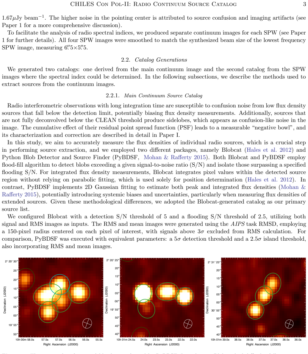
The argument is carried by four widely separated VLA spectral windows (central frequencies 1.063, 1.447, 1.703, and 1.831 GHz) that are imaged jointly for the main continuum and separately for spectral indices. The main catalog combines the Blobcat extractor's model-independent integrated photometry with PyBDSF's Gaussian-fitting deblending of confused sources, adopting Blobcat for single sources and PyBDSF for blended ones. Spectral indices are derived from power-law fits to the four matched-beam SPW images, and the $S/N \ge 20$ reliability criterion is established empirically by showing that extreme indices ($\alpha < -1.5$ or $\alpha > 1.0$) disappear once that threshold is applied.
What would settle it
Run the Monte-Carlo completeness test with extended sources of realistic sizes (e.g., 2--3 times the beam) at flux densities of 50 to 500 $\mu\mathrm{Jy}$; if their recovery fraction is substantially below the point-source completeness curve, the Section 4.5 source counts are underestimated and the catalog's bright-end correction is wrong.
Extended reading notes
Core claim
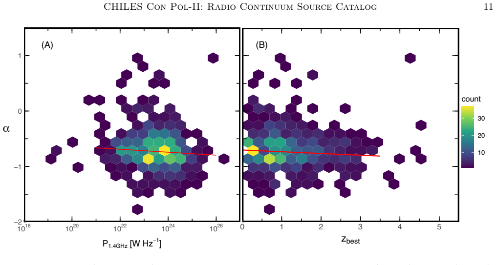
The central discovery is a confusion-limited, microjansky-depth 1.4 GHz image of the COSMOS field together with a 1,678-source catalog. At the pointing center the RMS noise is $1.67\,\mu\mathrm{Jy\,beam^{-1}}$ with a $5.5''\times5.0''$ beam, and sources brighter than $S_{1.4\,\mathrm{GHz}} \ge 42\,\mu\mathrm{Jy}$ are mostly resolved. Spectral indices come from power-law fits across four spectral windows spanning 1.063--1.831 GHz, and the paper shows that a total $S/N$ of at least 20 is required before the measured indices stop being dominated by noise; the distribution then peaks at $\alpha = -0.706$ with a secondary concentration near $\alpha \approx 0$. Comparisons with MIGHTEE and VLA-COSMOS show flux-density agreement at high flux densities but reveal incompleteness and confusion in earlier faint catalogs.
Load-bearing premise
The completeness correction assumes inserted test sources are point-like Gaussians with the beam size, so it does not measure the recovery rate of extended sources; since resolved sources dominate above $42\,\mu\mathrm{Jy}$, the paper itself notes the source counts in the brighter regime may be slightly off.
Editorial extensions
If this is right
- The 1,678-source catalog, with redshifts for 95.3% of sources, provides a microjansky-depth reference for star-forming galaxies and AGN out to $z \sim 3$.
- Because resolved sources dominate above $42\,\mu\mathrm{Jy}$, the point-source-based completeness correction will undercount flux in the bright regime; the paper states its number counts there may be slightly off.
- Requiring total $S/N \ge 20$ removes noise-driven extreme spectral indices, so deep surveys can adopt this as a quality cut before interpreting spectral index distributions.
- Flux-density agreement with MIGHTEE and VLA-COSMOS at high flux densities, with clear discrepancies at the faint end, implies earlier published catalogs need completeness and confusion corrections before use in counts.
- The spectral index distribution peaking at $\alpha = -0.706$ and the absence of significant $\alpha$--$P_{1.4\,\mathrm{GHz}}$ or $\alpha$--$z$ correlations support a picture in which local conditions, not redshift-dependent effects, set the synchrotron spectra of sub-mJy sources.
Reading between the lines
- A natural extension, not done in the paper, is to repeat the completeness simulation with extended sources matched to the resolved population; if recovery drops, the bright-end counts in Table 4 would need upward revision.
- The paper's $S/N \ge 20$ threshold likely varies with spectral baseline: indices from the two closely spaced high-frequency windows (separated by only 128 MHz) will need a higher $S/N$ than the full four-window fit, which the paper mentions but does not quantify.
- Combining this catalog with higher-resolution 3 GHz COSMOS imaging could distinguish genuine extended emission from blending and sharpen both the resolved fractions and the faint source counts.
- The overdensity of about 30 sources near $z \approx 2.6$, noted as a possible proto-cluster, is a concrete target for spectroscopic follow-up to test whether the survey is tracing large-scale structure.
Signed reviews
Editorial analysis
A structured set of objections, weighed in public.
Referee Report
Summary. The paper presents the second paper of the CHILES Continuum & Polarization survey: a 1.4 GHz (effective 1.447 GHz) continuum image of a single VLA pointing in COSMOS with 1.67 µJy/beam RMS at the center and a 7σ catalog of 1,678 sources inside the 50% primary-beam area. The catalog is built from Blobcat as the primary extractor with PyBDSF used for deblending of 322 blended regions. The authors measure spectral indices by power-law fitting across four spectral windows, assert that S/N≥20 is required for a reliable index, derive radio powers using literature redshifts, compare flux densities with MIGHTEE and VLA-COSMOS, and present Euclidean-normalized source counts corrected for point-source completeness and effective area.
Significance. If the catalog is taken as a delivered resource, it is a valuable ultra-deep 1.4 GHz sample in COSMOS; the resolved/unresolved fraction and spectral index distributions are useful for studying the faint radio source population. The use of two independent extractors, the explicit deblending strategy, and external cross-checks against MIGHTEE and VLA-COSMOS are strengths, as is the consistency with independent P(D) model counts. The headline source counts, however, inherit an unquantified systematic from applying a point-source completeness correction to a source population that is dominated by resolved sources above 42 µJy.
major comments (2)
- [§2.3 and §4.5, Eq. (1)] The completeness correction applied to the source counts is measured from Monte Carlo injections of point-like 2D Gaussians at the synthesized beam size and is recovered with PyBDSF alone, while the production catalog is based on Blobcat detections with PyBDSF used only to deblend sources (§2.2.1). Figure 4 and Table 2 show that resolved sources dominate at S1.4GHz ≥ 42 µJy, and Eq. (1) divides every count bin by C_j (point-source completeness) and the effective area without any correction for the different recovery rate or flux measurement bias of extended sources. The text acknowledges that the brighter counts 'might be slightly off' but gives no bound, so the 40–150 µJy and 150–500 µJy bins in Table 4 and their comparison in Figure 10 carry an unquantified systematic. Please add an extended-source completeness/recovery simulation, restrict the counts to a regime where the point-source completeness assumption is valid, or provide a quantitative systematic error budget for these bins.
- [§4.2.1 and Figure 5] The S/N≥20 threshold for a 'reliable' spectral index is inferred only from the disappearance of extreme values in the observed distribution. Because the measurement noise in the four SPW fits is the quantity at issue, an injection/recovery simulation, or at least a bootstrap or leave-one-SPW-out validation on the real data, is needed to demonstrate that the fitted index is unbiased and that the quoted α uncertainties are accurate at S/N~20. This is particularly relevant because spectral indices are derived for 96.2% of sources, many using only two SPWs, including the closely spaced SPW3/4 pair.
minor comments (5)
- [§2.2.2 and Table 1] Please state explicitly whether the SPW spectral index fits use peak or integrated flux densities; the fitting text mentions ϵ_peak, but the table lists both quantities.
- [§4.2.1 and Figure 5] The text says the histogram peak is at α = −0.725 while the panel labels and other text give α = −0.706; please reconcile these values.
- [§3.2] The text contains the typo 'Sptizer' where 'Spitzer' is meant, and the Figure 7 caption contains 'Deroved' instead of 'Derived'.
- [References] The companion 'Paper 1' is cited as 'Luber et al. in press' and appears in Figure 10 as 'CCP (Luber et al. 2024)', but no bibliographic entry for this work is included in the reference list.
- [§4.5, Eq. (1)] The summation in Eq. (1) uses j for C_j and A_j while the surrounding text defines C_i and A_i; please use consistent indices and clarify that S_mean is the weighted mean total flux density in each bin.
Circularity Check
No significant circularity: the catalog and derived properties are measured against independent external data, and no fitted parameter is fed back as a prediction.
full rationale
The paper's central products are a 7-sigma source catalog from a new VLA image and derived properties such as source sizes, spectral indices, radio powers, and source counts. The source counts in Eq. (1) are computed directly from the catalog flux densities, measured completeness fractions, and primary-beam effective areas; no count model or fitted parameter is used as an input to the detection or photometry, so the counts are not forced by construction. The completeness simulation in Sec. 2.3 is a recovery test on injected point-source Gaussians, and while the paper itself concedes that resolved sources dominate above about 42 microJy and that the brighter-bin counts 'might be slightly off,' this is an acknowledged systematic limitation rather than a circular reduction, because the correction does not presuppose the final counts. Spectral indices are computed from flux densities measured in the four SPW images with a power-law fit; the S/N >= 20 reliability threshold is inferred from the data, and no fitted spectral index is used to re-derive the catalog. Comparisons are made against independent external surveys, including MIGHTEE and VLA-COSMOS, and against literature source counts. The P(D) model line in Fig. 10 is taken from companion Paper I by the same team, but it is used only as a comparison curve, not as the basis for the individual source catalog or the binned counts, and its known dependence on the chosen pixel range is disclosed in the text. The self-citations to Paper I for calibration, imaging, and P(D) analysis are methodological references rather than load-bearing derivations of this paper's empirical claims. No equation reduces to its own input, and no fitted parameter is renamed as a prediction; therefore the circularity score is 0.
Assumptions & free parameters
free parameters (1)
- Power-law spectral index model S ~ nu^alpha =
fitted per source, mode -0.706
assumptions (3)
- domain assumption The radio flux density follows a power law across the four SPW frequencies.
- domain assumption The completeness of point-source recovery, measured with PyBDSF on inserted Gaussians, applies to the full catalog including resolved sources.
- domain assumption The RMS noise image used for source detection accurately represents the local noise.
Cite this review
Pith. "Pith review of The CHILES Continuum & Polarization Survey-II: Radio Continuum Source Catalog and Radio Properties." pith.science (2026). https://pith.science/paper/CC2MSJJ5
@misc{pith2026250420200,
  author       = {Pith},
  title        = {Pith review of: The CHILES Continuum & Polarization Survey-II: Radio Continuum Source Catalog and Radio Properties},
  year         = {2026},
  howpublished = {\url{https://pith.science/paper/CC2MSJJ5}},
  note         = {Machine review of arXiv:2504.20200}
}
abstract
The COSMOS HI Large Extragalactic Survey (CHILES) Continuum & Polarization (CHILES Con Pol) survey is an ultra-deep continuum imaging study of the COSMOS field conducted using the Karl G. Jansky Very Large Array. We obtained 1000 hours of L-band ($\lambda = 20$ cm) observations across four spectral windows (1.063-1.831 GHz) on a single pointing and produced a confusion limited image with an apparent RMS noise of 1.67 $\mu$Jy beam$^{-1}$ with a synthesized beam of 5$.\!\!^{\prime\prime}$5$\times$5$.\!\!^{\prime\prime}$0. This paper reports a 1.4 GHz radio continuum source catalog containing 1678 sources detected above 7$\sigma$ (flux densities greater than 11.7 $\mu$Jy), identified using two independent source extraction programs applied to the Stokes $I$ image. Resolved sources dominate at flux density S$_{1.4GHz} \ge 42 $\mu$Jy. Radio spectral index for each source was derived using a power-law fit across the four spectral windows, and we found that a robust spectral index measurement requires a total signal-to-noise ratio of at least 20. Comparisons with previous 1.4 GHz radio continuum surveys show good overall consistency, but evidence for a high degree of catalog incompleteness and the effects of source confusion are evident for some of the earlier studies.
Figures


Figures from the paper (7 more)




Reference graph
Works this paper leans on
-
[1]
2002, MNRAS, 329, 355, doi: 10.1046/j.1365-8711.2002.04988.x
Arnouts, S., Moscardini, L., Vanzella, E., et al. 2002, MNRAS, 329, 355, doi: 10.1046/j.1365-8711.2002.04988.x
arXiv 2002
-
[2]
Bell, E. F. 2003, ApJ, 586, 794, doi: 10.1086/367829
doi:10.1086/367829 2003
-
[3]
Dwarakanath, K. S. 2018, ApJ, 865, 39, doi: 10.3847/1538-4357/aad698
-
[4]
Blandford, R. D., & K¨ onigl, A. 1979, ApJ, 232, 34, doi: 10.1086/157262
doi:10.1086/157262 1979
-
[5]
M., Rawlings, S., & Willott, C
Blundell, K. M., Rawlings, S., & Willott, C. J. 1999, AJ, 117, 677, doi: 10.1086/300721
doi:10.1086/300721 1999
-
[6]
2003, A&A, 403, 857, doi: 10.1051/0004-6361:20030382
Bondi, M., Ciliegi, P., Zamorani, G., et al. 2003, A&A, 403, 857, doi: 10.1051/0004-6361:20030382
-
[7]
Brammer, G. B., van Dokkum, P. G., & Coppi, P. 2008, ApJ, 686, 1503, doi: 10.1086/591786
doi:10.1086/591786 2008
-
[8]
Briggs, D. S. 1995, in American Astronomical Society Meeting Abstracts, Vol. 187, American Astronomical Society Meeting Abstracts, 112.02 Calistro Rivera, G., Williams, W. L., Hardcastle, M. J., et al. 2017, MNRAS, 469, 3468, doi: 10.1093/mnras/stx1040
Show all 57 references
-
[9]
L., Perley, R
Carilli, C. L., Perley, R. A., Dreher, J. W., & Leahy, J. P. 1991, ApJ, 383, 554, doi: 10.1086/170813
1991 doi
-
[10]
M., Cooray, A., Capak, P., et al
Casey, C. M., Cooray, A., Capak, P., et al. 2015, ApJL, 808, L33, doi: 10.1088/2041-8205/808/2/L33
2015 doi
-
[11]
2003, A&A, 398, 901, doi: 10.1051/0004-6361:20021721
Ciliegi, P., Zamorani, G., Hasinger, G., et al. 2003, A&A, 398, 901, doi: 10.1051/0004-6361:20021721
2003 doi
-
[12]
2021, CARTA: The Cube Analysis and Rendering Tool for Astronomy, 2.0.0, Zenodo, doi: 10.5281/zenodo.4905459
Comrie, A., Wang, K.-S., Hsu, S.-C., et al. 2021, CARTA: The Cube Analysis and Rendering Tool for Astronomy, 2.0.0, Zenodo, doi: 10.5281/zenodo.4905459
2021 doi
-
[13]
Condon, J. J. 1992, ARA&A, 30, 575, doi: 10.1146/annurev.aa.30.090192.003043 de Zotti, G., Massardi, M., Negrello, M., & Wall, J. 2010, A&A Rv, 18, 1, doi: 10.1007/s00159-009-0026-0
1992
-
[14]
P., Andrews, S
Driver, S. P., Andrews, S. K., da Cunha, E., et al. 2018, MNRAS, 475, 2891, doi: 10.1093/mnras/stx2728
2018 doi
-
[15]
1986, A&A, 168, 17
Eckart, A., Witzel, A., Biermann, P., et al. 1986, A&A, 168, 17
1986
-
[16]
1981, Zeitschrift f¨ ur Wahrscheinlichkeitstheorie und Verwandte Gebiete, 57, 453, doi: 10.1007/BF01025868
Freedman, D., & Diaconis, P. 1981, Zeitschrift f¨ ur Wahrscheinlichkeitstheorie und Verwandte Gebiete, 57, 453, doi: 10.1007/BF01025868
1981 doi
-
[17]
B., Hales, C
Gim, H. B., Hales, C. A., Momjian, E., & Yun, M. S. 2015, in American Astronomical Society Meeting Abstracts, Vol. 225, American Astronomical Society Meeting Abstracts, 143.40
2015
-
[18]
B., Yun, M
Gim, H. B., Yun, M. S., Owen, F. N., et al. 2019, ApJ, 875, 80, doi: 10.3847/1538-4357/ab1011
2019 doi
-
[19]
L., Whittam, I
Hale, C. L., Whittam, I. H., Jarvis, M. J., et al. 2023, MNRAS, 520, 2668, doi: 10.1093/mnras/stac3320
2023 doi
-
[20]
A., Murphy, T., Curran, J
Hales, C. A., Murphy, T., Curran, J. R., et al. 2012, MNRAS, 425, 979, doi: 10.1111/j.1365-2966.2012.21373.x
2012
-
[21]
2018, ApJ, 858, 77, doi: 10.3847/1538-4357/aabacf
Hasinger, G., Capak, P., Salvato, M., et al. 2018, ApJ, 858, 77, doi: 10.3847/1538-4357/aabacf
2018 doi
-
[22]
M., & Best, P
Heckman, T. M., & Best, P. N. 2014, ARA&A, 52, 589, doi: 10.1146/annurev-astro-081913-035722
2014 doi
-
[23]
2017, MNRAS, 471, 1634, doi: 10.1093/mnras/stx1672
Herrero-Illana, R., P´ erez-Torres, M.´A., Randriamanakoto, Z., et al. 2017, MNRAS, 471, 1634, doi: 10.1093/mnras/stx1672
2017 doi
-
[24]
J., Hale, C
Heywood, I., Jarvis, M. J., Hale, C. L., et al. 2022, MNRAS, 509, 2150, doi: 10.1093/mnras/stab3021
2022 doi
-
[25]
J., et al
Ilbert, O., Arnouts, S., McCracken, H. J., et al. 2006, A&A, 457, 841, doi: 10.1051/0004-6361:20065138
2006 doi
-
[26]
Jamrozy, M., Konar, C., Machalski, J., & Saikia, D. J. 2008, MNRAS, 385, 1286, doi: 10.1111/j.1365-2966.2007.12772.x
2008
-
[27]
2016, in MeerKAT Science: On the Pathway to the SKA, 6, doi: 10.22323/1.277.0006 Jim´ enez-Andrade, E
Jarvis, M., Taylor, R., Agudo, I., et al. 2016, in MeerKAT Science: On the Pathway to the SKA, 6, doi: 10.22323/1.277.0006 Jim´ enez-Andrade, E. F., Murphy, E. J., Momjian, E., et al. 2024, ApJ, 972, 89, doi: 10.3847/1538-4357/ad5b5c
2016 doi
-
[28]
M., Dunkley, J., et al
Komatsu, E., Smith, K. M., Dunkley, J., et al. 2011, ApJS, 192, 18, doi: 10.1088/0067-0049/192/2/18
2011 doi
-
[29]
K., Taylor, G
Kumar, P., Schinzel, F. K., Taylor, G. B., et al. 2023, ApJ, 945, 129, doi: 10.3847/1538-4357/acba93
2023 doi
-
[30]
C., Thompson, T
Lacki, B. C., Thompson, T. A., & Quataert, E. 2010, ApJ, 717, 1, doi: 10.1088/0004-637X/717/1/1
2010 doi
-
[31]
A., & Peacock, J
Laing, R. A., & Peacock, J. A. 1980, MNRAS, 190, 903, doi: 10.1093/mnras/190.4.903
1980 doi
-
[32]
J., Lutz, D., et al
Magnelli, B., Ivison, R. J., Lutz, D., et al. 2015, A&A, 573, A45, doi: 10.1051/0004-6361/201424937
2015 doi
-
[33]
M., Condon, J
Matthews, A. M., Condon, J. J., Cotton, W. D., & Mauch, T. 2021, ApJ, 909, 193, doi: 10.3847/1538-4357/abdd37
2021 doi
-
[34]
D., Condon, J
Mauch, T., Cotton, W. D., Condon, J. J., et al. 2020, ApJ, 888, 61, doi: 10.3847/1538-4357/ab5d2d
2020 doi
-
[35]
2008, A&A Rv, 15, 67, doi: 10.1007/s00159-007-0008-z
Miley, G., & De Breuck, C. 2008, A&A Rv, 15, 67, doi: 10.1007/s00159-007-0008-z
2008 doi
-
[36]
A., & Mead, A
Miller, L., Peacock, J. A., & Mead, A. R. G. 1990, MNRAS, 244, 207 18 Gim et al
1990
-
[37]
2015, PyBDSF: Python Blob Detection and Source Finder
Mohan, N., & Rafferty, D. 2015, PyBDSF: Python Blob Detection and Source Finder. http://ascl.net/1502.007
2015
-
[38]
J., Condon, J
Murphy, E. J., Condon, J. J., Alberdi, A., et al. 2018, in Astronomical Society of the Pacific Conference Series, Vol. 517, Science with a Next Generation Very Large Array, ed. E. Murphy, 421
2018
-
[39]
F., Taylor, A
Ocran, E. F., Taylor, A. R., Vaccari, M., Ishwara-Chandra, C. H., & Prandoni, I. 2020, MNRAS, 491, 1127, doi: 10.1093/mnras/stz2954 Orr` u, E., Murgia, M., Feretti, L., et al. 2010, A&A, 515, A50, doi: 10.1051/0004-6361/200913837
2020 doi
-
[40]
Owen, F. N. 2018, ApJS, 235, 34, doi: 10.3847/1538-4365/aab4a1
2018 doi
-
[41]
N., & Morrison, G
Owen, F. N., & Morrison, G. E. 2008, AJ, 136, 1889, doi: 10.1088/0004-6256/136/5/1889
2008 doi
-
[42]
H., et al
Prandoni, I., Parma, P., Wieringa, M. H., et al. 2006, A&A, 457, 517, doi: 10.1051/0004-6361:20054273 R Core Team. 2013, R: A Language and Environment for Statistical Computing, R Foundation for Statistical
2006 doi
-
[43]
Rau, U., Bhatnagar, S., & Owen, F. N. 2016, AJ, 152, 124, doi: 10.3847/0004-6256/152/5/124
2016 doi
-
[44]
Rees, M. J. 1967, MNRAS, 136, 279, doi: 10.1093/mnras/136.3.279
1967 doi
-
[45]
2022, A&A, 663, A153, doi: 10.1051/0004-6361/202039750
Retana-Montenegro, E. 2022, A&A, 663, A153, doi: 10.1051/0004-6361/202039750
2022 doi
-
[46]
N., Tasse, C., et al
Sabater, J., Best, P. N., Tasse, C., et al. 2021, A&A, 648, A2, doi: 10.1051/0004-6361/202038828
2021 doi
-
[47]
B., Salvato, M., Aussel, H., et al
Sanders, D. B., Salvato, M., Aussel, H., et al. 2007, ApJS, 172, 86, doi: 10.1086/517885
2007 doi
-
[48]
T., Bondi, M., et al
Schinnerer, E., Sargent, M. T., Bondi, M., et al. 2010, ApJS, 188, 384, doi: 10.1088/0067-0049/188/2/384
2010 doi
-
[49]
Schleicher, D. R. G., & Beck, R. 2013, A&A, 556, A142, doi: 10.1051/0004-6361/201321707
2013 doi
-
[50]
2022, MNRAS, 514, 4343, doi: 10.1093/mnras/stac1504 Smolˇ ci´ c, V., Schinnerer, E., Finoguenov, A., et al
Sinha, A., Basu, A., Datta, A., & Chakraborty, A. 2022, MNRAS, 514, 4343, doi: 10.1093/mnras/stac1504 Smolˇ ci´ c, V., Schinnerer, E., Finoguenov, A., et al. 2007, ApJS, 172, 295, doi: 10.1086/516583 Smolˇ ci´ c, V., Novak, M., Bondi, M., et al. 2017a, A&A, 602, A1, doi: 10.10...
2022 doi
-
[51]
1992, MNRAS, 259, 413
Sutherland, W., & Saunders, W. 1992, MNRAS, 259, 413
1992
-
[52]
J., et al
Tasse, C., Shimwell, T., Hardcastle, M. J., et al. 2021, A&A, 648, A1, doi: 10.1051/0004-6361/202038804
2021 doi
-
[53]
Tielens, A. G. G. M., Miley, G. K., & Willis, A. G. 1979, A&AS, 35, 153 van der Vlugt, D., Algera, H. S. B., Hodge, J. A., et al. 2021, ApJ, 907, 5, doi: 10.3847/1538-4357/abcaa3
1979 doi
-
[54]
R., Kauffmann, O
Weaver, J. R., Kauffmann, O. B., Ilbert, O., et al. 2022, ApJS, 258, 11, doi: 10.3847/1538-4365/ac3078
2022 doi
-
[55]
H., Riley, J
Whittam, I. H., Riley, J. M., Green, D. A., et al. 2013, MNRAS, 429, 2080, doi: 10.1093/mnras/sts478
2013 doi
-
[56]
H., Prescott, M., Hale, C
Whittam, I. H., Prescott, M., Hale, C. L., et al. 2024, MNRAS, 527, 3231, doi: 10.1093/mnras/stad3307
2024 doi
-
[57]
S., Reddy, N
Yun, M. S., Reddy, N. A., & Condon, J. J. 2001, ApJ, 554, 803, doi: 10.1086/323145
2001 doi
Reviewed August 16, 2026 · model on record in the stance chip above.
Discussion (0). Continue with ORCID to comment.