REVIEW 3 major objections 6 minor 35 references
An Improved Autoencoder Conjugacy Network to Learn Chaotic Maps
T0 review · 3 major / 6 minor · reviewed 2026-08-06 · deepseek-v4-flash
Pith's one-line read An autoencoder that hard-codes the analytic conjugacy between the tent map and the logistic map in its latent space predicts continuous one-dimensional chaotic maps with lower error than a learned-conjugacy autoencoder, a feedforward…
desk verdict A modest but legitimate stability fix for autoencoder conjugacy in 1D chaotic maps; the printed loss equations don't match the forward model, so it needs a correction before it's reproducible. read the letter →
The pith
A machine-rendered reading of the paper's core claim, the machinery that carries it, and where it could break.
The reading
What carries the argument
The load-bearing object is the exact homeomorphism $\phi(x)=\frac{2}{\pi}\arcsin(\sqrt{x})$ from $[0,1]$ to $[0,1]$, with inverse $\phi^{-1}(y)=\sin^2(\pi y/2)$, which conjugates the logistic map $L(x)=4x(1-x)$ to the tent map $T(y)=2y$ for $y<1/2$ and $T(y)=2(1-y)$ for $y\ge 1/2$. The network hard-codes $\phi$ and $\phi^{-1}$ as a fixed layer around the tent map, so the latent propagator is exactly logistic; the only learned parts are the encoder $h$ and decoder $h^{-1}$, which need to approximate the conjugacy between the target map and the logistic map. This removes the need to learn a quadratic latent map with data-dependent coefficients and is what the paper credits for the stability and accuracy gains on continuous maps.
What would settle it
Train the proposed model on a continuous map that is provably conjugate to the logistic map but whose conjugacy is deliberately hard for a one-hidden-layer encoder to approximate, for example a conjugacy with a very steep derivative; if the one-step mean-squared error no longer beats the best learned-conjugacy baseline, the claim that hard-coding the tent–logistic conjugacy drives the improvement would be refuted. Reproducing Table 1 with independent code and the same fixed hyperparameters would also settle the comparison, since the reported gains are numerical rather than proven bounds.
Extended reading notes
Core claim
The central claim is that a chaotic map can be learned more accurately by representing it as $U = h^{-1} \circ \phi^{-1} \circ T \circ \phi \circ h$, where $T$ is the tent map, $\phi$ is the known analytic conjugacy, and $h,h^{-1}$ are encoder/decoder approximants of the unknown conjugacy between $U$ and the logistic map. Because $\phi^{-1}\circ T\circ\phi$ is exactly the logistic map at $r=4$, the latent variable $y=h(x)$ evolves under the true logistic dynamics rather than under an approximate learned map of the form $c_1 y + c_2 y^2$. The paper's numerical evidence is Table 1: for the continuous maps tested, the proposed model achieves one-step mean-squared errors around $10^{-6}$, lower than the learned-conjugacy autoencoder, the feedforward network, and the physics-informed network, and it avoids the vanishing-gradient failures that afflict the learned latent logistic map for some parameter choices. For the discontinuous doubling and Pomeau–Manneville maps the paper reports the reverse ordering, with the physics-informed network giving the lowest error, which it attributes to the absence of a true conjugacy.
Load-bearing premise
The load-bearing premise is that each target map can be converted into the logistic map by a coordinate change that a small neural-network encoder can learn from a uniform sample of points; the doubling and Pomeau–Manneville maps do not satisfy this premise, and the paper's own table shows the accuracy advantage disappears there.
Editorial extensions
If this is right
- For any continuous one-dimensional map known to be conjugate to the logistic map, the same fixed tent–logistic layer can be reused and only the outer encoder/decoder need retraining.
- The hard-coded conjugacy removes the vanishing-gradient failures that occur in the learned-conjugacy baseline, whose Table 1 entries are marked '-' for several parameter choices.
- Training needs only a uniform sample of initial conditions and one map step, not a long reliable orbit, which sidesteps the main data-generation problem for chaotic systems.
- A user who needs accurate orbits of piecewise maps such as the doubling or Pomeau–Manneville map should expect the physics-informed network, not this architecture, to give the lower error.
Reading between the lines
- Extending beyond the paper's tested cases, if the mechanism generalizes, target maps with known conjugacies beyond the logistic family could be swapped into the same template by replacing $\phi$ with the corresponding exact conjugacy, making the architecture a modular recipe rather than a single-map fix.
- The failure pattern on discontinuous maps suggests a testable refinement: split the domain at discontinuity points and apply the conjugacy layer branchwise, since the paper's figures indicate errors concentrate at the sharp transitions.
- One could also measure whether the benefit comes specifically from the tent map's piecewise linearity or from having any exactly known latent law, by substituting a different exactly solvable conjugate pair and comparing errors.
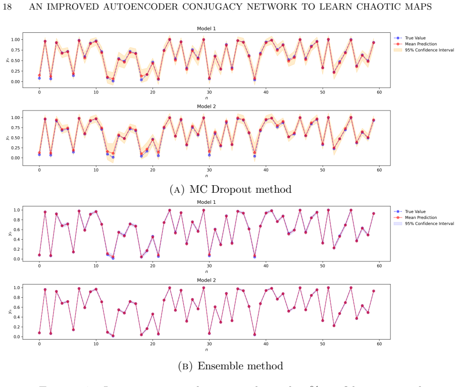
- The paper's uncertainty analysis indicates that MC-dropout uncertainty is sensitive to hidden dimension, so a fair comparison of architectures should report error bars across hidden widths, not just at one tuned width.
Signed reviews
Editorial analysis
A structured set of objections, weighed in public.
Referee Report
Summary. The paper proposes an autoencoder architecture (Model 1) for one-dimensional chaotic maps in which the encoder and decoder are learned while the latent layer is a fixed analytic conjugacy between the tent map T(x)=2x for x<1/2 and T(x)=2(1-x) for x≥1/2 and the logistic map L(x)=4x(1-x). The predicted map is written as Ũ(x)=h^{-1}(φ^{-1}(T(φ(h(x))))), with φ(x)=(2/π) arcsin(√x). The paper compares this model against the learned-conjugacy autoencoder of Bramburger et al., a feedforward network, and a physics-informed neural network on five one-dimensional maps, reporting in Table 1 that the new model has the lowest prediction error on the continuous maps (logistic, custom, Katsura–Fukuda) and that a PINN has the lowest error on the piecewise maps (doubling, Pomeau–Manneville). The limitations section acknowledges that the architecture relies on an assumed conjugacy between the target map and the logistic map.
Significance. If the numerical results are reproducible, the contribution is a useful engineering improvement to conjugate-mapping autoencoders: using the closed-form tent-logistic conjugacy in the latent space removes the learned quadratic latent map L(y)=c1y+c2y^2 of Bramburger et al., avoids the reported vanishing-gradient failures, and improves accuracy on continuous maps that are conjugate to the logistic map. The paper is honest about the main limitation in §5.2, makes code and data available, and does not overclaim a new theoretical result. The strength of the empirical claim is currently undermined by the mis-specified loss equations and the absence of repeated-run statistics; these are fixable in revision.
major comments (3)
- [§3.3, Eqs. (10)–(11)] The loss functions do not match the forward model in Eq. (9). Eq. (9) defines Ũ(x)=h^{-1}(φ^{-1}(T(φ(h(x))))), so the prediction loss should compare U(x) with h^{-1}(φ^{-1}(T(φ(h(x))))). As written, Eq. (11) uses h(U(x)) as the argument to the conjugacy layer, and Eq. (10) reconstructs U(x) rather than x. Implementing the text literally would train a different network, one that maps U(x) through the conjugacy layer, rather than the claimed x↦U(x) autoencoder. Please correct Eqs. (10) and (11) and verify that the public code agrees with the corrected expressions.
- [Table 1, §5.1] The headline comparisons are reported as single point estimates with no error bars, no standard deviations over random seeds, and no significance tests. Since the margins over Model 2 are often only a factor of 2–10, and since the text itself notes sensitivity to initialization, the claim that Model 1 provides the lowest prediction error is not statistically supported. Report mean and standard deviation over at least 5–10 independent training runs, or provide the ensemble and MC-dropout intervals described in §4.5 for the Table 1 numbers.
- [§3.1, §5, Figures 5–6] The training-data construction is stated inconsistently. Section 3 says the approach uses the first time step of a large uniform sample of initial conditions, but Section 5 and Figures 5–6 say the models used sequences of 300 in length, with 80% of the data allocated for training. Clarify whether each sample is a pair (x_i, U(x_i)) with x_i drawn uniformly, or a temporal window from a single orbit, since this determines whether the method actually avoids long-orbit generation and is essential for re-implementation.
minor comments (6)
- [§4.5, Eq. (16)] The Monte Carlo dropout mean is written as (1/T) Σ_{i=1}^N; the index N is not defined. It should be (1/T) Σ_{i=1}^T or the dummy index should be defined.
- [§5.2 and Abstract] The abstract says the method is demonstrated on both continuous and piecewise chaotic one-dimensional maps, but Table 1 shows the PINN (Model 4) achieves the lowest error on both piecewise maps. Please adjust the wording to avoid overstating the piecewise-map results.
- [§4.1–4.2] For the custom and Katsura–Fukuda maps, the text cites references for conjugacy or equivalence to the logistic map but does not give the conjugating function or its domain; providing these would let readers check the architectural assumption.
- [Figures 5 and 6 captions] The captions say deep learning models in 3, presumably meaning Models 1–4; the reference is incomplete and should be corrected.
- [§4.5] The dropout probability and ensemble size used for Figures 7–11 are not specified; add these settings to Table 2 or to the text.
- [Table 1] The '-' entries for Model 2 are attributed to vanishing gradients, but no criterion is given for when this occurs; specify, for example, NaNs or failure to decrease loss below a threshold.
Circularity Check
No material circularity: the latent tent/logistic conjugacy is a known analytic homeomorphism, not a fitted parameter, and predictions are supervised against independently generated map values.
full rationale
The paper's central claim is an architecture improvement, not a derivation of the conjugacy. The function phi(x) = (2/pi) arcsin(sqrt(x)) is standard and parameter-free, with an explicit inverse, and it is hard-coded in the latent space (Eqs. 3, 4, 8, 9) rather than fit to data. The encoder and decoder h and h^{-1} are learned from uniform samples, and the prediction targets U(x) are generated directly from the defining formulas of the logistic, custom, Katsura-Fukuda, doubling, and Pomeau-Manneville maps. For the logistic map itself, the internal latent map equals the target by design, so the experiment partly checks whether h can learn the identity; this is an intended inductive bias, not a fitted parameter renamed as a prediction. Comparisons to Bramburger et al., FNN, and PINN use fixed hyperparameters and external baselines, and no load-bearing claim rests on a self-citation or an imported uniqueness theorem. The limitations section candidly states that the assumed conjugacy fails for piecewise maps, and Table 1 indeed shows larger errors there. One non-circular correctness concern should be noted: the loss expressions in Eqs. (10)-(11) substitute U(x) for x inside h and phi, contradicting the forward model in Eq. (9); if taken literally, the training objective does not implement the described x -> U(x) map. This is a reproducibility or typographical issue, not circularity, and does not change the circularity score.
Assumptions & free parameters
free parameters (3)
- Hidden layer width =
256 (continuous maps), 64 (Pomeau-Manneville)
- Learning rate =
0.005 (continuous maps), 0.001 (piecewise maps)
- Training epochs =
1000 (continuous maps), 2000 (piecewise maps)
assumptions (5)
- standard math phi(x) = (2/pi) arcsin(sqrt x) defines a topological conjugacy between the tent map T_2 and the logistic map L_4 on [0,1]
- domain assumption The custom map (eq 12) is conjugate to the logistic map
- domain assumption The Katsura-Fukuda map with r=0.5 is equivalent to the logistic map
- domain assumption The doubling map is semiconjugate to the logistic map
- ad hoc to paper A feedforward encoder/decoder pair can be trained to approximate the (semi)conjugacy h and its inverse sufficiently accurately for the composed map to reproduce the target
Cite this review
Pith. "Pith review of An Improved Autoencoder Conjugacy Network to Learn Chaotic Maps." pith.science (2026). https://pith.science/paper/G2AOL272
@misc{pith2026250709835,
  author       = {Pith},
  title        = {Pith review of: An Improved Autoencoder Conjugacy Network to Learn Chaotic Maps},
  year         = {2026},
  howpublished = {\url{https://pith.science/paper/G2AOL272}},
  note         = {Machine review of arXiv:2507.09835}
}
read the original abstract
We introduce a method for learning chaotic maps using an improved autoencoder neural network that incorporates a conjugacy layer in the latent space. The added conjugacy layer transforms nonlinear maps into a simple piecewise linear map (the tent map) whilst enforcing dynamical principles of well-known and defective conjugacy functions that increase the accuracy and stability of the learned solution. We demonstrate the method's effectiveness on both continuous and piecewise chaotic one-dimensional maps and numerically illustrate improved performance over related traditional and recently emerged deep learning architectures.
Figures


Figures from the paper (8 more)




Reference graph
Works this paper leans on
-
[1]
Extremes and recurrence in dynamical systems
Valerio Lucarini, Davide Faranda, Jorge Miguel Milhazes de Freitas, Mark Holland, Tobias Kuna, Matthew Nicol, Mike Todd, Sandro Vaienti, et al. Extremes and recurrence in dynamical systems. John Wiley & Sons, 2016
work page 2016
-
[2]
Ashesh Chattopadhyay, Pedram Hassanzadeh, and Devika Subramanian. Data- driven predictions of a multiscale lorenz 96 chaotic system using machine-learning methods: Reservoir computing, artificial neural network, and long short-term mem- ory network. Nonlinear Processes in Geophysics, 27(3):373–389, 2020
work page 2020
-
[3]
Classification of chaotic time series with deep learning
Nicolas Boull´ e, Vassilios Dallas, Yuji Nakatsukasa, and D Samaddar. Classification of chaotic time series with deep learning. Physica D: Nonlinear Phenomena , 403: 132261, 2020
work page 2020
-
[4]
Long- term prediction of chaotic systems with machine learning
Huawei Fan, Junjie Jiang, Chun Zhang, Xingang Wang, and Ying-Cheng Lai. Long- term prediction of chaotic systems with machine learning. Physical Review Research, 2(1):012080, 2020
work page 2020
-
[5]
Controlling nonlinear dynamical sys- tems into arbitrary states using machine learning
Alexander Haluszczynski and Christoph R¨ ath. Controlling nonlinear dynamical sys- tems into arbitrary states using machine learning. Scientific reports, 11(1):12991, 2021
work page 2021
-
[6]
Modeling of nonlinear system based on deep learning framework
Xiangjun Jin, Jie Shao, Xin Zhang, Wenwei An, and Reza Malekian. Modeling of nonlinear system based on deep learning framework. Nonlinear Dynamics , 84: 1327–1340, 2016
work page 2016
-
[7]
Deep learning for universal linear embeddings of nonlinear dynamics
Bethany Lusch, J Nathan Kutz, and Steven L Brunton. Deep learning for universal linear embeddings of nonlinear dynamics. Nature communications, 9(1):4950, 2018
2018
-
[8]
Jaideep Pathak, Brian Hunt, Michelle Girvan, Zhixin Lu, and Edward Ott. Model- free prediction of large spatiotemporally chaotic systems from data: A reservoir computing approach. Physical review letters , 120(2):024102, 2018
work page 2018
Show all 35 references
-
[9]
New results for prediction of chaotic systems using deep recurrent neural networks
Jos´ e de Jes´ us Serrano-P´ erez, Guillermo Fern´ andez-Anaya, Salvador Carrillo-Moreno, and Wen Yu. New results for prediction of chaotic systems using deep recurrent neural networks. Neural Processing Letters, 53:1579–1596, 2021
2021
-
[10]
Neural machine-based forecasting of chaotic dynamics
Rui Wang, Eugenia Kalnay, and Balakumar Balachandran. Neural machine-based forecasting of chaotic dynamics. Nonlinear Dynamics, 98(4):2903–2917, 2019
2019
-
[11]
Modeling chaotic sys- tems: Dynamical equations vs machine learning approach
Tongfeng Weng, Huijie Yang, Jie Zhang, and Michael Small. Modeling chaotic sys- tems: Dynamical equations vs machine learning approach. Communications in Non- linear Science and Numerical Simulation , 114:106452, 2022
2022
-
[12]
Physics-informed neu- ral networks: A deep learning framework for solving forward and inverse problems involving nonlinear partial differential equations
Maziar Raissi, Paris Perdikaris, and George E Karniadakis. Physics-informed neu- ral networks: A deep learning framework for solving forward and inverse problems involving nonlinear partial differential equations. Journal of Computational physics , 378:686–707, 2019
2019
-
[13]
Physica D, 2025
Machine learning and dynamical systems, guest editors: Boumediene hamzi, jeroen lamb, lorenzo livi, qianxiao li. Physica D, 2025. 24 AN IMPROVED AUTOENCODER CONJUGACY NETWORK TO LEARN CHAOTIC MAPS
2025
-
[14]
Linearly recurrent autoencoder networks for learning dynamics
Samuel E Otto and Clarence W Rowley. Linearly recurrent autoencoder networks for learning dynamics. SIAM Journal on Applied Dynamical Systems, 18(1):558–593, 2019
2019
-
[15]
Exploration and prediction of fluid dynamical systems using auto- encoder technology
Lionel Agostini. Exploration and prediction of fluid dynamical systems using auto- encoder technology. Physics of Fluids , 32(6), 2020
2020
-
[16]
Deep neural networks for nonlinear model order reduction of unsteady flows
Hamidreza Eivazi, Hadi Veisi, Mohammad Hossein Naderi, and Vahid Esfahanian. Deep neural networks for nonlinear model order reduction of unsteady flows. Physics of Fluids , 32(10), 2020
2020
-
[17]
Model reduction of dynamical systems on non- linear manifolds using deep convolutional autoencoders
Kookjin Lee and Kevin T Carlberg. Model reduction of dynamical systems on non- linear manifolds using deep convolutional autoencoders. Journal of Computational Physics, 404:108973, 2020
2020
-
[18]
Multi-level convolutional autoencoder networks for parametric prediction of spatio-temporal dynamics.Computer Methods in Applied Mechanics and Engineering , 372:113379, 2020
Jiayang Xu and Karthik Duraisamy. Multi-level convolutional autoencoder networks for parametric prediction of spatio-temporal dynamics.Computer Methods in Applied Mechanics and Engineering , 372:113379, 2020
2020
-
[19]
Machine learning approach to model order reduction of nonlinear systems via autoencoder and lstm networks
Thomas Simpson, Nikolaos Dervilis, and Eleni Chatzi. Machine learning approach to model order reduction of nonlinear systems via autoencoder and lstm networks. Journal of Engineering Mechanics , 147(10):04021061, 2021
2021
-
[20]
Learning physics constrained dynamics using autoencoders
Tsung-Yen Yang, Justinian Rosca, Karthik Narasimhan, and Peter J Ramadge. Learning physics constrained dynamics using autoencoders. Advances in Neural In- formation Processing Systems, 35:17157–17172, 2022
2022
-
[21]
Autoencoder neural net- works enable low dimensional structure analyses of microbial growth dynamics
Yasa Baig, Helena R Ma, Helen Xu, and Lingchong You. Autoencoder neural net- works enable low dimensional structure analyses of microbial growth dynamics. Na- ture Communications, 14(1):7937, 2023
2023
-
[22]
Data- driven discovery of coordinates and governing equations
Kathleen Champion, Bethany Lusch, J Nathan Kutz, and Steven L Brunton. Data- driven discovery of coordinates and governing equations. Proceedings of the National Academy of Sciences, 116(45):22445–22451, 2019
2019
-
[23]
Deep learning of conjugate mappings
Jason J Bramburger, Steven L Brunton, and J Nathan Kutz. Deep learning of conjugate mappings. Physica D: Nonlinear Phenomena , 427:133008, 2021
2021
-
[24]
Relaxing conjugacy to fit modeling in dynamical systems
Joseph D Skufca and Erik M Bollt. Relaxing conjugacy to fit modeling in dynamical systems. Physical Review E—Statistical, Nonlinear, and Soft Matter Physics , 76(2): 026220, 2007
2007
-
[25]
A concept of homeomorphic defect for defin- ing mostly conjugate dynamical systems
Joseph D Skufca and Erik M Bollt. A concept of homeomorphic defect for defin- ing mostly conjugate dynamical systems. Chaos: An Interdisciplinary Journal of Nonlinear Science, 18(1), 2008
2008
-
[26]
On comparing dynamical systems by defective conjugacy: A symbolic dynamics interpretation of commuter functions
Erik M Bollt and Joseph D Skufca. On comparing dynamical systems by defective conjugacy: A symbolic dynamics interpretation of commuter functions. Physica D: Nonlinear Phenomena, 239(10):579–590, 2010
2010
-
[27]
Theorem to generate independently and uniformly distributed chaotic key stream via topologically conjugated maps of tent map
Zheng Guang Xu, Qing Tian, and Li Tian. Theorem to generate independently and uniformly distributed chaotic key stream via topologically conjugated maps of tent map. Mathematical Problems in Engineering , 2012(1):619257, 2012. AN IMPROVED AUTOENCODER CONJUGACY NETWORK TO LEARN...
2012
-
[28]
Quadratic function chaotic system and its application on digital image encryption
Hongfeng Guo, Xin Zhang, Xinyao Zhao, Hang Yu, and Li Zhang. Quadratic function chaotic system and its application on digital image encryption. IEEE Access, 8: 55540–55549, 2020
2020
-
[29]
Behavior of logistic map and some of its conjugate maps
Ahmad Tedi Ruslan, Marwan, and Qurratul Aini. Behavior of logistic map and some of its conjugate maps. In AIP Conference Proceedings, volume 2641, page 020002. AIP Publishing LLC, 2022
2022
-
[30]
Differentiable conjugacies for one- dimensional maps
Paul Glendinning and David JW Simpson. Differentiable conjugacies for one- dimensional maps. In International Conference on Difference Equations and Ap- plications, pages 115–130. Springer, 2022
2022
-
[31]
An introduction to dynamical systems and chaos, volume 1
GC Layek et al. An introduction to dynamical systems and chaos, volume 1. Springer, 2015
2015
-
[32]
Survival and weak chaos
Sean Nee. Survival and weak chaos. Royal Society open science , 5(5):172181, 2018
2018
-
[33]
Dropout: a simple way to prevent neural networks from overfitting
Nitish Srivastava, Geoffrey Hinton, Alex Krizhevsky, Ilya Sutskever, and Ruslan Salakhutdinov. Dropout: a simple way to prevent neural networks from overfitting. The journal of machine learning research , 15(1):1929–1958, 2014
1929
-
[34]
Dropout as a bayesian approximation: Repre- senting model uncertainty in deep learning
Yarin Gal and Zoubin Ghahramani. Dropout as a bayesian approximation: Repre- senting model uncertainty in deep learning. In international conference on machine learning, pages 1050–1059. PMLR, 2016
2016
-
[35]
Simple and scalable predictive uncertainty estimation using deep ensembles
Balaji Lakshminarayanan, Alexander Pritzel, and Charles Blundell. Simple and scalable predictive uncertainty estimation using deep ensembles. Advances in neural information processing systems, 30, 2017. The University of Queensland School of Mathematics and Physics Email addre...
2017
Reviewed August 6, 2026 · model on record in the stance chip above.
Discussion (0). Continue with ORCID to comment.