REVIEW 2 major objections 6 minor 45 references
Deep Learning for High Speed Optical Coherence Elastography with a Fiber Scanning Endoscope
T0 review · 2 major / 6 minor · reviewed 2026-08-05 · deepseek-v4-flash
Pith's one-line read A 2.2 mm endoscope combined with end-to-end deep learning can map soft-tissue elasticity in real time, without knowing wave direction.
desk verdict A genuinely new endoscopic elastography probe with a mostly sound validation; the absolute accuracy numbers rest on an unverified ground-truth transfer, so treat them as provisional rather than proven. read the letter →
The pith
A machine-rendered reading of the paper's core claim, the machinery that carries it, and where it could break.
The reading
What carries the argument
The load-bearing object is the conical (pseudo 3D+t) scan pattern generated by deflecting the imaging fiber with a piezoelectric tube at 5.05 kHz, yielding a circular trajectory that samples a propagating wave field in three spatial-plus-time dimensions. The second component is a spatio-temporal DenseNet—a real-valued densely connected convolutional network with about 110,000 parameters—that takes phase-difference volumes (depth × lateral × time) and regresses Young's modulus. The network learns the mapping implicitly, absorbing the probe's scan geometry and the unknown wave directions during training on phantoms whose stiffness is labeled by indentation tests, so no explicit velocity estima
What would settle it
Indent the exact phantom regions imaged by the endoscope immediately after scanning and compare the co-located Young's modulus with the network's predictions; if the mean absolute error against those directly measured values substantially exceeds the reported 4.48±3.63 kPa, the phantom-to-phantom transfer assumption fails.
Extended reading notes
Core claim
The central claim is that a fiber-scanning endoscope with a conical scan pattern, together with an end-to-end spatio-temporal convolutional network, can convert raw optical-coherence phase data of a diffuse multi-frequency wave field directly into quantitative Young's modulus estimates, without knowing the excitation position or wave propagation direction. The paper reports that for pseudo 3D+t scanning the mean absolute error is 4.48±3.63 kPa, roughly a four-fold improvement over the conventional 2D FFT approach (19.75±21.82 kPa), and that the estimates are spatially uniform across the field of view. It further claims this is the first application of a fiber scanning endoscope to shear wave
Load-bearing premise
The Young's modulus labels that train and evaluate the network are measured on separate cross-sectional gelatin cylinders, and the reported errors assume those indentation values exactly match the stiffness of the phantoms actually imaged.
Editorial extensions
If this is right
- A 2.2 mm endoscope can generate localized elasticity maps at roughly 14 Hz, compatible with continuous scanning during minimally invasive surgery.
- The method removes the need to know or calibrate the excitation location and wave propagation direction, simplifying probe design and deployment.
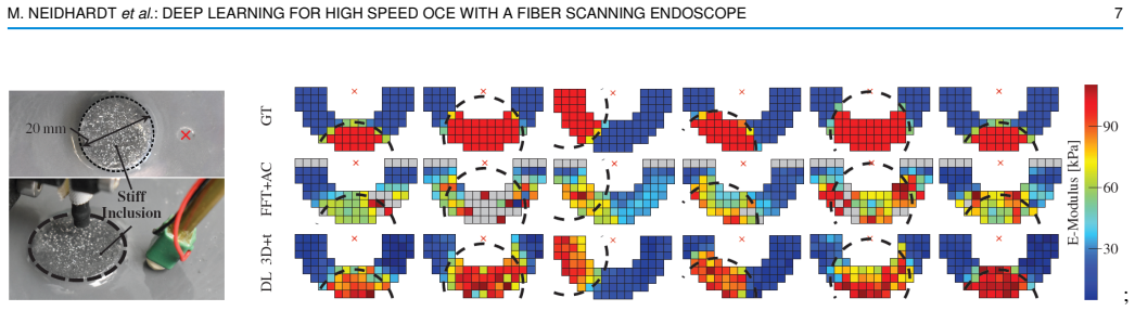
- On phantoms with a stiff inclusion, deep learning estimates segment the inclusion with DICE 0.91±0.03, compared with 0.64±0.10 for the conventional method.
- Because the network is trained end-to-end, the same architecture could be retrained on clinical labels to perform tissue classification directly, avoiding indentation tests.
- Ex-vivo porcine heart results suggest the approach can distinguish adipose and muscle tissue, pointing toward surgical navigation applications.
Reading between the lines
- The reported accuracy depends on the assumption that the imaged phantoms have exactly the same stiffness as the separately indented replicate phantoms; a co-located indentation on the imaged samples would be a stronger test of the mapping.
- Since the network implicitly absorbs the probe's scan geometry and wave-field statistics, changing the scan pattern, probe hand-built imperfections, or excitation frequencies would likely require retraining or fine-tuning before the error figures carry over.
- The multi-frequency excitation and diffuse wave fields suggest the network may be able to estimate viscoelastic or frequency-dependent properties, not just a single Young's modulus, if the training labels are extended.
- The approach could transfer to other excitation sources, such as instrument-integrated piezoelectric actuators, as long as the resulting wave fields are captured by the same conical scanning geometry.
Signed reviews
Editorial analysis
A structured set of objections, weighed in public.
Referee Report
Summary. The paper presents a fiber scanning endoscope (FSE) with a 2.2 mm outer diameter that acquires high-speed OCT images of propagating shear wave fields in either 2D+t (line) or pseudo 3D+t (conical) scan patterns. The authors propose an end-to-end spatio-temporal DenseNet that takes raw phase data (or ST maps) and directly regresses Young's modulus, avoiding the need for explicit wave-direction estimation, triggering, or spatial calibration of the excitation position. They compare this against a conventional FFT-based phase-velocity estimator with and without angle correction, using leave-one-phantom-out cross-validation on homogeneous gelatin phantoms. The headline result is that the pseudo-3D DL method achieves a mean absolute error of 4.48±3.63 kPa, compared with 19.75±21.82 kPa for the conventional FFT method and 11.33±12.78 kPa for the angle-corrected version. A held-out test on inclusion phantoms reports a DICE score of 0.91±0.03, and ex-vivo porcine heart images demonstrate the feasibility of mapping adipose and muscle tissue. The central claim is that a robust, local, contactless, non-directional elasticity estimate is feasible with a miniature FSE.
Significance. If the reported accuracy holds, this is a significant contribution to interventional elastography. The work is, to the best of the reviewer's knowledge, the first application of a fiber scanning endoscope to shear wave OCE, and the deep learning pipeline eliminates several practical bottlenecks of conventional methods: it does not require knowledge of the excitation position, does not need triggered acquisition, and avoids explicit wave-direction reconstruction. The experimental design is a clear strength: the leave-one-phantom-out cross-validation, the held-out inclusion-phantom test, the systematic variation of imaging position with a robot, and the reported real-time inference rate (about 14 Hz) all support the practical feasibility claim. The DL approach also consistently outperforms the conventional baseline, even when the baseline is given the excitation position and a test-set-fitted calibration, which makes the relative comparison conservative and credible. The paper is clearly of interest to the IEEE TMI readership, but the absolute accuracy claims require further validation.
major comments (2)
- [Section II-F / III / Table I] The ground-truth Young's moduli used for both training and evaluation come from indentation tests on separately manufactured cylindrical phantoms, not from the phantoms that were actually imaged. The text states this explicitly: 'indentation tests performed on additionally manufactured cylindrical gelatin phantoms containing the same gelatin to water ratio.' Thus the reported MAEs (e.g., 4.48±3.63 kPa) are errors relative to nominal concentration-level labels. Batch-to-batch variation in gelatin preparation, temperature history, or aging could bias every reported error, and the magnitude of this bias is unquantified. Since the absolute error is the paper's headline quantitative claim, this is a load-bearing issue. The authors should either provide co-located mechanical measurements on the imaged phantoms (or samples from the same batch) or explicitly reframe the claims as relative to a c
- [Section II-D] The conventional baseline's linear calibration E = k·v + q with k=24.2, q=-16.4 is stated to be obtained by minimizing the absolute error between FFT estimates and indentation values, apparently on the same evaluation data used to report the final errors. This is a test-set calibration, giving the baseline an advantage that the DL method does not receive. While the DL method still outperforms the baseline, the comparison is not on a methodologically equal footing. The calibration should be performed within each cross-validation fold, or at minimum the authors should explicitly state that this calibration is a best-case upper bound for the conventional approach and quantify the sensitivity of the coefficients.
minor comments (6)
- [Table II, G15% row] The entry '12.13±79.1' appears to be a typographical error; the standard deviation 79.1 is implausibly large compared with the surrounding values. Likely it should be '12.13±7.91'.
- [Figure 7 / Results] The reported precision value '0.94 ± 2.51' for the FFT+AC method is impossible: precision cannot exceed 1, and a standard deviation of 2.51 is invalid for a quantity constrained to [0,1]. This is likely a typo (e.g., 0.94±0.25) and must be corrected.
- [Section II-E] The sentence 'As a baseline, we used densely connected neural networks [31]' is vague because the paper immediately describes a custom DenseNet. Please clarify whether the literature baseline refers to the architecture family or a specific prior implementation, and describe any modifications made here.
- [Section II-G] The description 'We trained in total four networks for each fold while randomly choosing a phantom from each gelatin concentration for validation' is unclear. It should explain why four networks are trained (e.g., four random validation splits) and how their predictions are combined or selected.
- [Section III] The sentence 'apart from the 3% gelatin concentration the MAE is always best when the FSE is operated in pseudo 3D+t scan mode' is contradicted by Table II, where the pseudo 3D+t method has the lowest MAE at all concentrations, including G3%. This should be corrected.
- [Section IV] The sentence 'The size of our scan field already represents a typical laparoscopic image size of 53 × 40 mm at a working distance of 120 mm [44]' is confusing, as the scan field diameter is stated as approximately 1.5 mm. Please rephrase to clarify the intended comparison (e.g., the size of the elasticity map, the field of view after mosaicking, or the lateral resolution).
Circularity Check
Minor circularity in the conventional comparator's velocity-to-modulus calibration; the DL elasticity estimates themselves are trained on external indentation labels and validated on held-out phantoms, so the central claim is not circular.
-
fitted input called prediction
[Section II-D (Conventional Phase Velocity Estimation)]
"Exclusively for the conventional approach, we mapped the estimated velocities v to the Young’s Modulus E by a linear regression approach defined as E = k · v + q. We minimized the absolute error between estimates and define k = 24.2 and q = −16.4. This allows a fair comparison to our deep learning approach."
The coefficients k and q are obtained by minimizing the absolute error between the linear mapping output and the indentation-derived Young's modulus labels over the same homogeneous-phantom measurements whose errors are then reported in Table II. Therefore the conventional (FFT/FFT+AC) MAE is an in-sample calibration error of a fitted line, not an independent held-out prediction. The comparison 'DL 3D+t 4.48±3.63 kPa vs conventional 19.75±21.82 kPa' therefore pits a cross-validated deep network against a calibration-fitted baseline. Because the fit minimizes error, this bias favors the conventional comparator, so it does not inflate the central DL claim; nevertheless the 'fair comparison' framing is circular in this limited sense.
full rationale
The paper's central derivation is self-contained: the DenseNet is trained end-to-end on OCT phase data from homogeneous gelatin phantoms, with labels provided by uniaxial indentation tests performed on identically prepared cylindrical phantoms (Section II-F), and evaluated with a nested five-fold cross-validation leaving out whole phantoms of each concentration (Section II-G). The inclusion-phantom DICE evaluation is an additional generalization check on data not used in training. The indentation labels are external measurements, not constructed from the network outputs, so the DL error values do not reduce to the training inputs by construction. Self-citations ([7], [8], [14]) support the architecture and indentation protocol, but the present paper actually performs the phantom manufacture, indentation, and training; no uniqueness theorem or ansatz is imported as a load-bearing black box. The one genuine circular step is the conventional comparator's velocity-to-modulus linear regression, which is fitted by minimizing absolute error on the same data whose MAE is later reported. This is a secondary methodological flaw and not the paper's main claim. Separately, the transfer of indentation moduli from separately manufactured phantoms to the imaged phantoms is an unvalidated assumption, but that is an external-validity/correctness issue, not a circular derivation, so it does not raise the circularity score further.
Assumptions & free parameters
free parameters (3)
- Baseline linear calibration coefficients k, q =
k=24.2, q=-16.4
- FFT baseline band-pass and failure threshold =
center 400 Hz, band 200 Hz, 10% amplitude cutoff, v>10 m/s considered failed
- DL training hyperparameters =
lr=1e-5, batch=14, epochs=200, Adam, MSE
assumptions (4)
- domain assumption OCT phase differences between successive scan lines represent sub-resolution tissue displacement caused by the propagating wave field
- domain assumption Same-concentration gelatin phantoms have identical mechanical properties regardless of batch, temperature, and age
- domain assumption The spatio-temporal DenseNet trained on homogeneous phantoms generalizes to inclusion phantoms and ex-vivo tissue without retraining
- domain assumption The robot positioning (repeatability 0.01 mm) and the piezo excitation provide a stable and repeatable wave field across all 70 positions
Cite this review
Pith. "Pith review of Deep Learning for High Speed Optical Coherence Elastography with a Fiber Scanning Endoscope." pith.science (2026). https://pith.science/paper/SL6HQ2H4
@misc{pith2026250903193,
  author       = {Pith},
  title        = {Pith review of: Deep Learning for High Speed Optical Coherence Elastography with a Fiber Scanning Endoscope},
  year         = {2026},
  howpublished = {\url{https://pith.science/paper/SL6HQ2H4}},
  note         = {Machine review of arXiv:2509.03193}
}
read the original abstract
Tissue stiffness is related to soft tissue pathologies and can be assessed through palpation or via clinical imaging systems, e.g., ultrasound or magnetic resonance imaging. Typically, the image based approaches are not suitable during interventions, particularly for minimally invasive surgery. To this end, we present a miniaturized fiber scanning endoscope for fast and localized elastography. Moreover, we propose a deep learning based signal processing pipeline to account for the intricate data and the need for real-time estimates. Our elasticity estimation approach is based on imaging complex and diffuse wave fields that encompass multiple wave frequencies and propagate in various directions. We optimize the probe design to enable different scan patterns. To maximize temporal sampling while maintaining three-dimensional information we define a scan pattern in a conical shape with a temporal frequency of 5.05 kHz. To efficiently process the image sequences of complex wave fields we consider a spatio-temporal deep learning network. We train the network in an end-to-end fashion on measurements from phantoms representing multiple elasticities. The network is used to obtain localized and robust elasticity estimates, allowing to create elasticity maps in real-time. For 2D scanning, our approach results in a mean absolute error of 6.31+-5.76 kPa compared to 11.33+-12.78 kPa for conventional phase tracking. For scanning without estimating the wave direction, the novel 3D method reduces the error to 4.48+-3.63 kPa compared to 19.75+-21.82 kPa for the conventional 2D method. Finally, we demonstrate feasibility of elasticity estimates in ex-vivo porcine tissue.
Figures


Figures from the paper (6 more)



Reference graph
Works this paper leans on
-
[1]
J. M. Scott et al. , “Artificial neural networks for magnetic resonance elastography stiffness estimation in inhomogeneous materials,” Medical Image Analysis , vol. 63, p. 101710, 2020
work page 2020
-
[2]
M. S. Lee et al., “Prospective comparison among transient elastography, supersonic shear imaging, and ARFI imaging for predicting fibrosis in nonalcoholic fatty liver disease,” PloS one , vol. 12, no. 11, 2017
work page 2017
-
[3]
Automatic scanning of large tissue areas in neuro- surgery using optical coherence tomography,
M. Finke et al. , “Automatic scanning of large tissue areas in neuro- surgery using optical coherence tomography,” MRCAS, vol. 8, no. 3, pp. 327–336, 2012
work page 2012
-
[4]
Bimodal intravascular volumetric imaging combining oct and mpi,
S. Latus et al. , “Bimodal intravascular volumetric imaging combining oct and mpi,” Medical physics , vol. 46, no. 3, pp. 1371–1383, 2019
work page 2019
-
[5]
Automatic plaque detection in ivoct pullbacks using convolutional neural networks,
N. Gessert et al. , “Automatic plaque detection in ivoct pullbacks using convolutional neural networks,” IEEE TMI, vol. 38, pp. 426–434, 2018
work page 2018
-
[6]
Estimation of shear wave velocity in gelatin phantoms utilizing PhS-SSOCT,
R. K. Manapuram et al. , “Estimation of shear wave velocity in gelatin phantoms utilizing PhS-SSOCT,” Laser Physics , vol. 22, no. 9, pp. 1439–1444, 2012
work page 2012
-
[7]
Deep learning for high speed optical coherence elastog- raphy,
M. Neidhardt, M. Bengs, S. Latus, M. Schluter, T. Saathoff, and A. Schlaefer, “Deep learning for high speed optical coherence elastog- raphy,” in 2020 IEEE 17th ISBI . IEEE, 2020, pp. 1583–1586
work page 2020
-
[8]
4D deep learning for real-time volumetric optical co- herence elastography,
M. Neidhardt, M. Bengs, S. Latus, M. Schl ¨uter, T. Saathoff, and A. Schlaefer, “4D deep learning for real-time volumetric optical co- herence elastography,” IJCARS, vol. 16, no. 1, pp. 23–27, 2021
work page 2021
Show all 45 references
-
[9]
Microscope-integrated intraoperative OCT with electrically tunable focus and heads-up display for imaging of ophthalmic surgical maneuvers,
Y . K. Tao, S. K. Srivastava, and J. P. Ehlers, “Microscope-integrated intraoperative OCT with electrically tunable focus and heads-up display for imaging of ophthalmic surgical maneuvers,” Biomed. Opt. Express , vol. 5, no. 6, pp. 1877–1885, 2014
2014
-
[10]
Development of novel imaging probe for optical/acoustic radiation imaging (OARI),
O. A. Ejofodomi, V . Zderic, and J. M. Zara, “Development of novel imaging probe for optical/acoustic radiation imaging (OARI),” Medical physics, vol. 40, no. 11, p. 111910, 2013
2013
-
[11]
Quantitative optical coherence elastography based on fiber-optic probe for in situ measurement of tissue mechanical proper- ties,
Y . Qiu et al. , “Quantitative optical coherence elastography based on fiber-optic probe for in situ measurement of tissue mechanical proper- ties,” Biomed. Opt. Express , vol. 7, no. 2, pp. 688–700, 2016
2016
-
[12]
Intravascular optical coherence elastography,
T. Wang et al. , “Intravascular optical coherence elastography,” Biomed. Opt. Express, vol. 13, no. 10, p. 5418, 2022
2022
-
[13]
An approach for needle based optical coherence elastography measurements,
S. Latus et al. , “An approach for needle based optical coherence elastography measurements,” in Proceedings MICCAI 2017 . Springer, 2017, pp. 655–663
2017
-
[14]
Ultrasound shear wave elasticity imaging with spatio-temporal deep learning,
M. Neidhardt et al. , “Ultrasound shear wave elasticity imaging with spatio-temporal deep learning,” IEEE. Trans. Biomed. Eng. , 2022
2022
-
[15]
A focused air-pulse system for optical-coherence- tomography-based measurements of tissue elasticity,
S. Wang et al. , “A focused air-pulse system for optical-coherence- tomography-based measurements of tissue elasticity,” Laser Physics Letters, vol. 10, no. 7, p. 075605, 2013
2013
-
[16]
Two-dimensional (2d) dy- namic vibration optical coherence elastography (dv-oce) for evaluating mechanical properties: a potential application in tissue engineering,
H.-C. Liu, P. Kijanka, and M. W. Urban, “Two-dimensional (2d) dy- namic vibration optical coherence elastography (dv-oce) for evaluating mechanical properties: a potential application in tissue engineering,” Biomedical Optics Express , vol. 12, no. 3, pp. 1217–1235, 2021
2021
-
[17]
Integrated optical coherence tomography and multielement ultrasound transducer probe for shear wave elasticity imaging of moving tissues,
A. B. Karpiouk, D. J. VanderLaan, K. V . Larin, and S. Y . Emelianov, “Integrated optical coherence tomography and multielement ultrasound transducer probe for shear wave elasticity imaging of moving tissues,” J. Biomed. Opt. , vol. 23, no. 10, pp. 1–7, 2018
2018
-
[18]
Miniature probe for mapping mechanical properties of vascular lesions using acoustic radiation force optical coherence elastography,
Y . Qu et al. , “Miniature probe for mapping mechanical properties of vascular lesions using acoustic radiation force optical coherence elastography,” Sci. Rep. , vol. 7, no. 1, p. 4731, 2017
2017
-
[19]
Portable optical coherence elastography system with flexible and phase stable common path optical fiber probe,
A. Parmar, G. Sharma, S. Sharma, and K. Singh, “Portable optical coherence elastography system with flexible and phase stable common path optical fiber probe,” IEEE Access, vol. 9, pp. 56 041–56 048, 2021
2021
-
[20]
A miniature dual-fiber probe for quantitative optical coherence elastography,
S. Latus et al. , “A miniature dual-fiber probe for quantitative optical coherence elastography,” IEEE. Trans. Biomed. Eng. , vol. PP, 2023
2023
-
[21]
Forward-viewing resonant fiber-optic scanning endoscope of appropriate scanning speed for 3d OCT imaging,
L. Huo, J. Xi, Y . Wu, and X. Li, “Forward-viewing resonant fiber-optic scanning endoscope of appropriate scanning speed for 3d OCT imaging,” Optics Express, vol. 18, no. 14, pp. 14 375–14 384, 2010
2010
-
[22]
Endoscopic forward-viewing optical coherence tomog- raphy and angiography with MHz swept source,
K. Liang et al., “Endoscopic forward-viewing optical coherence tomog- raphy and angiography with MHz swept source,” Optics Letters, vol. 42, no. 16, pp. 3193–3196, 2017
2017
-
[23]
High-speed fiber scanning endoscope for volumetric multi-megahertz optical coherence tomography,
H. Schulz-Hildebrandt et al., “High-speed fiber scanning endoscope for volumetric multi-megahertz optical coherence tomography,” Opt. Lett. , vol. 43, no. 18, pp. 4386–4389, 2018
2018
-
[24]
Full-range fourier domain optical coherence tomography imaging probe with a magnetic-driven resonant fiber cantilever,
Y . Huang, “Full-range fourier domain optical coherence tomography imaging probe with a magnetic-driven resonant fiber cantilever,” Optical Engineering, vol. 50, no. 11, p. 119002, 2011
2011
-
[25]
Endoscopic optical coherence elastography using acoustic radiation force and a vibrating fiber,
K. Nakamura, R. Isago, and D. Koyama, “Endoscopic optical coherence elastography using acoustic radiation force and a vibrating fiber,” in AIP Conference Proceedings, vol. 1474, no. 1, 2012, pp. 247–250
2012
-
[26]
Arterial stiffness estimation by shear wave elastography: Validation in phantoms with mechanical testing,
E. Maksuti, E. Widman, D. Larsson, M. W. Urban, M. Larsson, and A. Bj¨allmark, “Arterial stiffness estimation by shear wave elastography: Validation in phantoms with mechanical testing,” Ultrasound Med Biol , vol. 42, no. 1, pp. 308–321, 2016
2016
-
[27]
Diffuse shear wave spectroscopy for soft tissue viscoelastic characterization,
S. Beuve, L. Kritly, S. Call ´e, and J.-P. Remenieras, “Diffuse shear wave spectroscopy for soft tissue viscoelastic characterization,” Ultrasonics, vol. 110, p. 106239, 2021
2021
-
[28]
Viscoelastic parameter estimation using simulated shear wave motion and convolutional neural networks,
L. Vasconcelos, P. Kijanka, and M. W. Urban, “Viscoelastic parameter estimation using simulated shear wave motion and convolutional neural networks,” Comput. Biol. Med. , vol. 133, p. 104382, 2021
2021
-
[29]
Swenet: a physics- informed deep neural network (pinn) for shear wave elastography,
Z. Yin, G.-Y . Li, Z. Zhang, Y . Zheng, and Y . Cao, “Swenet: a physics- informed deep neural network (pinn) for shear wave elastography,”IEEE Transactions on Medical Imaging , 2023
2023
-
[30]
Multiwave imaging and super resolution,
M. Fink and M. Tanter, “Multiwave imaging and super resolution,” Phys. Today, vol. 63, no. 2, pp. 28–33, 2010
2010
-
[31]
Densely connected convolutional networks,
G. Huang, Z. Liu, L. Van Der Maaten, and K. Q. Weinberger, “Densely connected convolutional networks,” in Proceedings IEEE CVPR , 2017, pp. 4700–4708
2017
-
[32]
Batch normalization: Accelerating deep network training by reducing internal covariate shift,
S. Ioffe and C. Szegedy, “Batch normalization: Accelerating deep network training by reducing internal covariate shift,” arXiv preprint arXiv:1502.03167, 2015
2015 arXiv
-
[33]
PyTorch Lightning,
W. Falcon and The PyTorch Lightning team, “PyTorch Lightning,” Mar
-
[34]
Morphometric analysis of white matter lesions in MR images: method and validation,
A. P. Zijdenbos, B. M. Dawant, R. A. Margolin, and A. C. Palmer, “Morphometric analysis of white matter lesions in MR images: method and validation,” IEEE TMI , vol. 13, no. 4, pp. 716–724, 1994
1994
-
[35]
Elastic modulus of muscle and tendon with shear wave ultrasound elastography: variations with different technical settings,
B. C. W. Kot, Z. J. Zhang, A. W. C. Lee, V . Y . F. Leung, and S. N. Fu, “Elastic modulus of muscle and tendon with shear wave ultrasound elastography: variations with different technical settings,” PLoS ONE , 2012
2012
-
[36]
Comparative analysis of indentation and magnetic resonance elastography for measuring viscoelastic properties,
Y . Chen, S. Qiu, Z. He, F. Yan, R. Li, and Y . Feng, “Comparative analysis of indentation and magnetic resonance elastography for measuring viscoelastic properties,” Acta Mech. Sin. , vol. 37, pp. 527–536, 2021
2021
-
[37]
Elastic properties of soft tissue- mimicking phantoms assessed by combined use of laser ultrasonics and low coherence interferometry,
C. Li, Z. Huang, and R. K. Wang, “Elastic properties of soft tissue- mimicking phantoms assessed by combined use of laser ultrasonics and low coherence interferometry,” Optics express, vol. 19, no. 11, pp. 10 153–10 163, 2011
2011
-
[38]
Determining elastic properties of skin by measuring surface waves from an impulse mechan- ical stimulus using phase-sensitive optical coherence tomography,
C. Li, G. Guan, R. Reif, Z. Huang, and R. K. Wang, “Determining elastic properties of skin by measuring surface waves from an impulse mechan- ical stimulus using phase-sensitive optical coherence tomography,” J. R. Soc. Interface , vol. 9, no. 70, pp. 831–841, 2012
2012
-
[39]
The biome- chanics of simple steatosis and steatohepatitis,
K. Parker, J. Ormachea, M. Drage, H. Kim, and Z. Hah, “The biome- chanics of simple steatosis and steatohepatitis,” Phys. Med. Biol., vol. 63, no. 10, p. 105013, 2018
2018
-
[40]
Feasibility of phase velocity imaging using multi frequency oscillation-shear wave elastography,
M. M. Hossain and E. E. Konofagou, “Feasibility of phase velocity imaging using multi frequency oscillation-shear wave elastography,” IEEE. Trans. Biomed. Eng , pp. 1–14, 2023
2023
-
[41]
High-speed markerless tissue motion tracking using volumetric optical coherence tomography images,
M. Schl ¨uter et al., “High-speed markerless tissue motion tracking using volumetric optical coherence tomography images,” in 2020 IEEE 17th ISBI. IEEE, 2020, pp. 1979–1982
2020
-
[42]
Stiffness and anisotropy effect on shear wave elastography: a phantom and in vivo renal study,
S. S. Leong et al. , “Stiffness and anisotropy effect on shear wave elastography: a phantom and in vivo renal study,” Ultrasound Med Biol , vol. 46, no. 1, pp. 34–45, 2020
2020
-
[43]
A modified da vinci surgical instrument for oce based elasticity estimation with deep learning,
M. Neidhardt, R. Mieling, S. Latus, M. Fischer, T. Maurer, and A. Schlaefer, “A modified da vinci surgical instrument for oce based elasticity estimation with deep learning,” in 2024 10th IEEE RAS/EMBS International Conference for BioRob . IEEE, 2024
2024
-
[44]
Characterization and in-vivo evalu- ation of a multi-resolution foveated laparoscope for minimally invasive surgery,
Y . Qin, H. Hua, and M. Nguyen, “Characterization and in-vivo evalu- ation of a multi-resolution foveated laparoscope for minimally invasive surgery,” Biomedical Optics Express, vol. 5, no. 8, pp. 2548–2562, 2014
2014
-
[2019]
Available: https://github.com/Lightning-AI/lightning
[Online]. Available: https://github.com/Lightning-AI/lightning
Reviewed August 5, 2026 · model on record in the stance chip above.
Discussion (0). Continue with ORCID to comment.