Novel Adaptive Schemes for Hyperbolic Conservation Laws
Pith reviewed 2026-05-18 14:44 UTC · model grok-4.3
The pith
Adaptive schemes for hyperbolic conservation laws use a smoothness indicator to apply overcompressive limiters only at contacts, Minmod2 elsewhere in rough zones, and a fifth-order scheme in smooth regions.
A machine-rendered reading of the paper's core claim, the machinery that carries it, and where it could break.
Core claim
The central claim is that a smoothness indicator can be used both to detect rough regions and to distinguish contact discontinuities within them, allowing the overcompressive limiter to be applied only where it sharpens contacts, the Minmod2 limiter to control oscillations in the remaining rough zones, and the fifth-order scheme to be used safely in smooth zones, thereby producing solutions that resolve shocks and contacts sharply while avoiding nonphysical structures.
What carries the argument
The smoothness indicator that both flags rough regions and classifies contact discontinuities, driving the switch among the overcompressive limiter, the Minmod2 limiter, and the quasi-linear fifth-order finite-difference scheme.
If this is right
- The adaptive schemes extend the earlier adaption strategy by adding a targeted distinction between contact discontinuities and other rough features.
- In smooth regions the fifth-order scheme can be used without risking oscillations near discontinuities.
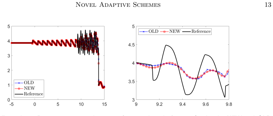
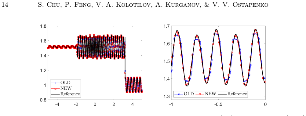
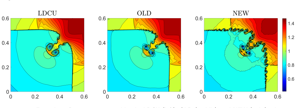
- Numerical examples confirm sharper resolution of both nonlinear shocks and linearly degenerate contacts compared with non-adaptive approaches.
- The same smoothness indicator serves dual purposes: region detection and discontinuity-type classification.
Where Pith is reading between the lines
- The approach could be tested on systems with multiple interacting waves to check whether the indicator still separates contacts reliably under wave collisions.
- Similar indicator-driven switching might be explored for other high-order reconstructions or for adaptive mesh refinement strategies.
- The method may reduce the need for manual tuning of limiter parameters in practical simulations of gas dynamics or shallow-water flows.
Load-bearing premise
The smoothness indicator must correctly identify contact discontinuities and separate them from other rough areas so that the appropriate limiter is chosen in each case.
What would settle it
A numerical test case in which the smoothness indicator mislabels a contact discontinuity, causing either visible oscillations or staircase structures to appear in the computed solution.
Figures


read the original abstract
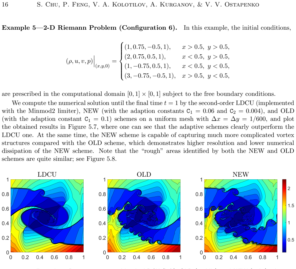
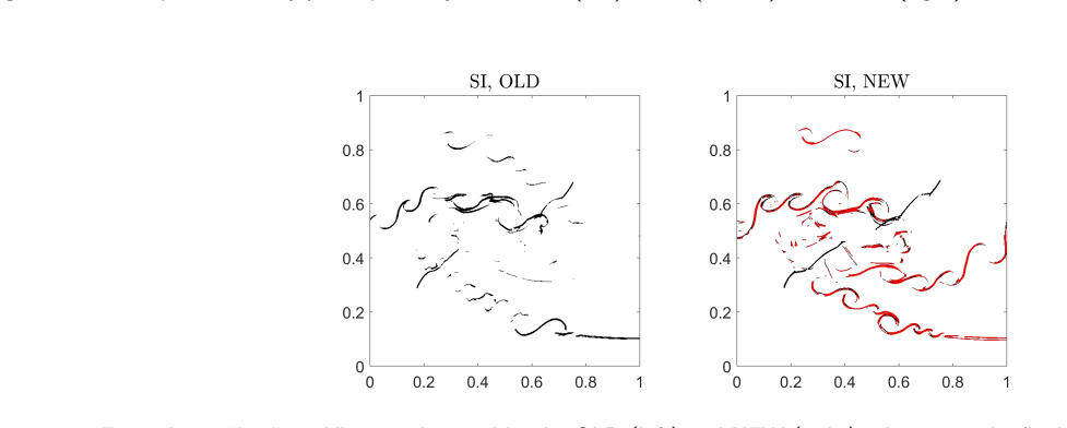
We introduce new adaptive schemes for the one- and two-dimensional hyperbolic systems of conservation laws. Our schemes are based on an adaption strategy recently introduced in [{\sc S. Chu, A. Kurganov, and I. Menshov}, Appl. Numer. Math., 209 (2025)]. As there, we use a smoothness indicator (SI) to automatically detect ``rough'' parts of the solution and employ in those areas the second-order finite-volume low-dissipation central-upwind scheme with an overcompressive limiter, which helps to sharply resolve nonlinear shock waves and linearly degenerate contact discontinuities. In smooth parts, we replace the limited second-order scheme with a quasi-linear fifth-order (in space and third-order in time) finite-difference scheme, recently proposed in [{\sc V. A. Kolotilov, V. V. Ostapenko, and N. A. Khandeeva}, Comput. Math. Math. Phys., 65 (2025)]. However, direct application of this scheme may generate spurious oscillations near ``rough'' parts, while excessive use of the overcompressive limiter may cause staircase-like nonphysical structures in smooth areas. To address these issues, we employ the same SI to distinguish contact discontinuities, treated with the overcompressive limiter, from other ``rough'' regions, where we switch to the dissipative Minmod2 limiter. Advantage of the resulting adaptive schemes are clearly demonstrated on a number of challenging numerical examples.
Editorial analysis
A structured set of objections, weighed in public.
Referee Report
Summary. The manuscript introduces adaptive schemes for one- and two-dimensional hyperbolic conservation laws. A smoothness indicator detects rough regions where a second-order central-upwind scheme with overcompressive limiter is applied to resolve shocks and contacts; a fifth-order finite-difference scheme is used in smooth regions. The same indicator further distinguishes contacts (overcompressive limiter) from other rough areas (Minmod2 limiter) to avoid oscillations and staircasing. Advantages are illustrated on several numerical test cases.
Significance. If the smoothness indicator reliably separates contacts, the adaptive combination could usefully merge high-order accuracy away from discontinuities with sharp, stable resolution at shocks and contacts. The work logically extends the cited prior schemes by the overlapping author groups and supplies visual evidence from challenging examples. Quantitative error norms, convergence rates, and baseline comparisons would substantially increase the significance.
major comments (1)
- [Section 3] The central adaptation logic relies on the smoothness indicator distinguishing contact discontinuities (for the overcompressive limiter) from other rough regions (for the Minmod2 limiter). No explicit formula, threshold, or additional sensor for this contact-specific classification is supplied, making it impossible to verify that misclassification will not reintroduce oscillations or staircasing and thereby undermine the claimed advantages.
minor comments (2)
- [Abstract] Abstract: the sentence beginning 'Advantage of the resulting adaptive schemes are' is grammatically incorrect and should be rephrased.
- [Numerical Experiments] The numerical examples would benefit from at least one table of L1 or L2 errors and observed convergence rates, even if only for the smooth test problems.
Simulated Author's Rebuttal
We thank the referee for the positive overall assessment of our work and for the constructive major comment, which helps us improve the clarity of the adaptation strategy. We address the point below and will revise the manuscript accordingly.
read point-by-point responses
-
Referee: [Section 3] The central adaptation logic relies on the smoothness indicator distinguishing contact discontinuities (for the overcompressive limiter) from other rough regions (for the Minmod2 limiter). No explicit formula, threshold, or additional sensor for this contact-specific classification is supplied, making it impossible to verify that misclassification will not reintroduce oscillations or staircasing and thereby undermine the claimed advantages.
Authors: We thank the referee for this observation. The manuscript states that the same smoothness indicator (SI) is used both to detect rough regions and to further classify contacts (treated with the overcompressive limiter) versus other discontinuities (treated with the Minmod2 limiter). However, we agree that Section 3 does not supply the explicit formula for the SI, the numerical thresholds that trigger the contact-specific switch, or any auxiliary sensor that prevents misclassification. In the revised manuscript we will add a dedicated subsection in Section 3 that presents (i) the precise mathematical definition of the SI, (ii) the threshold values and decision logic used to label a rough cell as a contact, and (iii) a brief discussion of how the chosen thresholds were calibrated on the test problems to avoid re-introduction of oscillations or staircasing. These additions will make the classification procedure fully reproducible and will directly address the referee’s concern. revision: yes
Circularity Check
Minor self-citations to overlapping-author prior schemes, but new adaptive distinction and external numerical tests remain independent
full rationale
The paper explicitly builds on an adaptation strategy and smoothness indicator from Chu, Kurganov, Menshov (2025) and a fifth-order scheme from Kolotilov, Ostapenko, Khandeeva (2025), both with author overlap. However, the central contribution is the novel routing logic that applies the same SI to send contact discontinuities to the overcompressive limiter while routing other rough regions to the Minmod2 limiter, then switches to the high-order scheme in smooth areas. This combination is presented as new and its advantages are shown via direct numerical experiments on external test problems rather than any fitted parameter, self-referential definition, or uniqueness theorem imported from the cited works. No equation or claim reduces by construction to the inputs; the self-citations supply reusable components without bearing the load of the reported resolution and oscillation-avoidance properties.
Axiom & Free-Parameter Ledger
axioms (1)
- domain assumption The smoothness indicator accurately detects rough parts and distinguishes contact discontinuities from other discontinuities or oscillations.
Lean theorems connected to this paper
-
IndisputableMonolith/Cost/FunctionalEquation.leanwashburn_uniqueness_aczel unclear?
unclearRelation between the paper passage and the cited Recognition theorem.
We employ the same SI to distinguish contact discontinuities, treated with the overcompressive limiter, from other “rough” regions, where we switch to the dissipative Minmod2 limiter.
-
IndisputableMonolith/Foundation/AlphaCoordinateFixation.leancostAlphaLog_fourth_deriv_at_zero unclear?
unclearRelation between the paper passage and the cited Recognition theorem.
E_ρ_j = |ρ_{j+1}−2ρ_j+ρ_{j−1}| / (|ρ_{j+1}−ρ_j|+|ρ_j−ρ_{j−1}|+ε(ρ_{j+1}+2ρ_j+ρ_{j−1}))
What do these tags mean?
- matches
- The paper's claim is directly supported by a theorem in the formal canon.
- supports
- The theorem supports part of the paper's argument, but the paper may add assumptions or extra steps.
- extends
- The paper goes beyond the formal theorem; the theorem is a base layer rather than the whole result.
- uses
- The paper appears to rely on the theorem as machinery.
- contradicts
- The paper's claim conflicts with a theorem or certificate in the canon.
- unclear
- Pith found a possible connection, but the passage is too broad, indirect, or ambiguous to say the theorem truly supports the claim.
Reference graph
Works this paper leans on
-
[1]
F. Ar \`a ndiga, A. Baeza, and R. Donat , Vector cell-average multiresolution based on H ermite interpolation , Adv. Comput. Math., 28 (2008), pp. 1--22
work page 2008
-
[2]
M. Ben-Artzi and J. Falcovitz , Generalized R iemann problems in computational fluid dynamics , vol. 11 of Cambridge Monographs on Applied and Computational Mathematics, Cambridge University Press, Cambridge, 2003
work page 2003
-
[3]
W. Boscheri and M. Dumbser , Arbitrary- L agrangian- E ulerian one-step WENO finite volume schemes on unstructured triangular meshes , Commun. Comput. Phys., 14 (2013), pp. 1174--1206
work page 2013
-
[4]
S. Z. Burstein and A. A. Mirin , Third order difference methods for hyperbolic equations , J. Comput. Phys., 5 (1970), pp. 547--571
work page 1970
-
[5]
A. Chertock, S. Chu, M. Herty, A. Kurganov, and M. Luk\'a c ov\'a-Medvi d ov\'a , Local characteristic decomposition based central-upwind scheme , J. Comput. Phys., 473 (2023). Paper No. 111718
work page 2023
-
[6]
A. Chertock, S. Chu, and A. Kurganov , Adaptive high-order A-WENO schemes based on a new local smoothness indicator , E. Asian. J. Appl. Math., 13 (2023), pp. 576--609
work page 2023
-
[7]
S. Chu, M. Herty, and A. Kurganov , Novel local characteristic decomposition based path-conservative central-upwind schemes , J. Comput. Phys., 524 (2025). Paper No. 113692
work page 2025
-
[8]
S. Chu, A. Kurganov, and I. Menshov , New adaptive low-dissipation central-upwind schemes , Appl. Numer. Math., 209 (2025), pp. 155--170
work page 2025
-
[9]
S. Chu, A. Kurganov, and R. Xin , Low-dissipation central-upwind schemes for compressible multifluids , J. Comput. Phys., 518 (2024). Paper No. 113311
work page 2024
-
[10]
S. Chu, A. Kurganov, and R. Xin , New low-dissipation central-upwind schemes. P art II , J. Sci. Comput., 193 (2025). Paper No. 33
work page 2025
- [11]
-
[12]
M. Dumbser, O. Zanotti, R. Loub\`ere, and S. Diot , A posteriori subcell limiting of the discontinuous G alerkin finite element method for hyperbolic conservation laws , J. Comput. Phys., 278 (2014), pp. 47--75
work page 2014
-
[13]
G. Fu and C.-W. Shu , A new troubled-cell indicator for discontinuous G alerkin methods for hyperbolic conservation laws , J. Comput. Phys., 347 (2017), pp. 305--327
work page 2017
-
[14]
Z. Gao, Q. Liu, J. S. Hesthaven, B.-S. Wang, W. S. Don, and X. Wen , Non-intrusive reduced order modeling of convection dominated flows using artificial neural networks with application to R ayleigh- T aylor instability , Commun. Comput. Phys., 30 (2021), pp. 97--123
work page 2021
-
[15]
A. Gelb and E. Tadmor , Spectral reconstruction of piecewise smooth functions from their discrete data , M2AN Math. Model. Numer. Anal., 36 (2002), pp. 155--175
work page 2002
-
[16]
A. Gelb and E. Tadmor , Adaptive edge detectors for piecewise smooth data based on the minmod limiter , J. Sci. Comput., 28 (2006), pp. 279--306
work page 2006
-
[17]
E. Godlewski and P.-A. Raviart , Numerical approximation of hyperbolic systems of conservation laws , Springer-Verlag, New York, second ed., 2021
work page 2021
-
[18]
S. Gottlieb, D. Ketcheson, and C.-W. Shu , Strong stability preserving R unge- K utta and multistep time discretizations , World Scientific Publishing Co. Pte. Ltd., Hackensack, NJ, 2011
work page 2011
-
[19]
S. Gottlieb, C.-W. Shu, and E. Tadmor , Strong stability-preserving high-order time discretization methods , SIAM Rev., 43 (2001), pp. 89--112
work page 2001
-
[20]
J.-L. Guermond, R. Pasquetti, and B. Popov , Entropy viscosity method for nonlinear conservation laws , J. Comput. Phys., 230 (2011), pp. 4248--4267
work page 2011
-
[21]
J. S. Hesthaven , Numerical methods for conservation laws: From analysis to algorithms , Comput. Sci. Eng. 18, SIAM, Philadelphia, 2018
work page 2018
- [22]
-
[23]
V. A. Kolotilov, A. A. Kurganov, V. V. Ostapenko, N. A. Khandeeva, and S. Chu , On the accuracy of shock-capturing schemes calculating gas-dynamic shock waves , Comput. Math. Math. Phys., 63 (2023), pp. 1341--1349
work page 2023
-
[24]
V. A. Kolotilov, V. V. Ostapenko, and N. A. Khandeeva , Fifth-order finite-difference scheme in space with increased accuracy in shock influence areas , Comput. Math. Math. Phys., 65 (2025), pp. 901--916
work page 2025
-
[25]
A. Kurganov and E. Tadmor , Solution of two-dimensional R iemann problems for gas dynamics without R iemann problem solvers , Numer. Methods Partial Differential Equations, 18 (2002), pp. 584--608
work page 2002
-
[26]
M. E. Ladonkina, O. A. Nekliudova, V. V. Ostapenko, and V. F. Tishkin , On the accuracy of discontinuous Galerkin method calculating gas-dynamic shock waves , Dokl. Math., 107 (2023), pp. 120--125
work page 2023
-
[27]
R. J. LeVeque , Finite Volume Methods for Hyperbolic Problems , Cambridge Texts in Appl. Math., Cambridge University Press, Cambridge, UK, 2002
work page 2002
- [28]
-
[29]
R. Liska and B. Wendrof , Comparison of several diference schemes on 1 D and 2 D test problems for the E uler equations , SIAM J. Sci. Comput., 25 (2003), pp. 995--1017
work page 2003
-
[30]
L\"ohner , An adaptive finite element scheme for transient problems in CFD , Comput
R. L\"ohner , An adaptive finite element scheme for transient problems in CFD , Comput. Methods Appl. Mech. Eng., 61 (1987), pp. 323--338
work page 1987
-
[31]
G. Puppo and M. Semplice , Numerical entropy and adaptivity for finite volume schemes , Commun. Comput. Phys., 10 (2011), pp. 1132--1160
work page 2011
-
[32]
J. Qiu and C.-W. Shu , On the construction, comparison, and local characteristic decomposition for high-order central WENO schemes , J. Comput. Phys., 183 (2002), pp. 187--209
work page 2002
-
[33]
J. Qiu and C.-W. Shu , A comparison of troubled-cell indicators for R unge- K utta discontinuous G alerkin methods using weighted essentially nonoscillatory limiters , SIAM J. Sci. Comput., 27 (2005), pp. 995--1013
work page 2005
-
[34]
V. V. Rusanov , Third-order accurate shock-capturing schemes for computing discontinuous solutions , Dokl. Akad. Nauk SSSR., 18 (1968), pp. 1303--1305
work page 1968
-
[35]
C. W. Schulz-Rinne , Classifcation of the R iemann problem for two-dimensional gas dynamics , SIAM J. Math. Anal., 24 (1993), pp. 76--88
work page 1993
-
[36]
C. W. Schulz-Rinne, J. P. Collins, and H. M. Glaz , Numerical solution of the R iemann problem for two-dimensional gas dynamics , SIAM J. Sci. Comput., 14 (1993), pp. 1394--1414
work page 1993
- [37]
-
[38]
C.-W. Shu , Essentially non-oscillatory and weighted essentially non-oscillatory schemes for hyperbolic conservation laws , in Advanced numerical approximation of nonlinear hyperbolic equations ( C etraro, 1997), vol. 1697 of Lecture Notes in Math., Springer, Berlin, 1998, pp. 325--432
work page 1997
-
[39]
C.-W. Shu , Essentially non-oscillatory and weighted essentially non-oscillatory schemes , Acta Numer., 5 (2020), pp. 701--762
work page 2020
- [40]
-
[41]
Osher , Efficient implementation of essentially nonoscillatory shock-capturing schemes
C.-W Shu and S. Osher , Efficient implementation of essentially nonoscillatory shock-capturing schemes. II , J. Comput. Phys., 83 (1989), pp. 32--78
work page 1989
-
[42]
E. F. Toro , Riemann solvers and numerical methods for fluid dynamics: A practical introduction , Springer-Verlag, Berlin, Heidelberg, third ed., 2009
work page 2009
-
[43]
M. J. Vuik and J. K. Ryan , Automated parameters for troubled-cell indicators using outlier detection , SIAM J. Sci. Comput., 38 (2016), pp. A84--A104
work page 2016
-
[44]
W. Wang, C.-W. Shu, H. C. Yee, D. V. Kotov, and B. Sj\" o green , High order finite difference methods with subcell resolution for stiff multispecies discontinuity capturing , Commun. Comput. Phys., 17 (2015), pp. 317--336
work page 2015
-
[45]
X. Wen, W. S. Don, Z. Gao, and J. S. Hesthaven , An edge detector based on artificial neural network with application to hybrid compact- WENO finite difference scheme , J. Sci. Comput., 83 (2020). Paper No. 49
work page 2020
-
[46]
P. Woodward and P. Colella , The numerical solution of two-dimensional fluid flow with strong shocks , J. Comput. Phys., 54 (1988), pp. 115--173
work page 1988
-
[47]
Zheng , Systems of conservation laws
Y. Zheng , Systems of conservation laws. Two-dimensional Riemann problems , Progress in Nonlinear Differential Equations and their Applications, Birkh\" a user Boston, Inc., Boston, MA, 2001
work page 2001
-
[48]
" write newline "" before.all 'output.state := FUNCTION fin.entry add.period write newline FUNCTION new.block output.state before.all = 'skip after.block 'output.state := if FUNCTION not #0 #1 if FUNCTION and 'skip pop #0 if FUNCTION or pop #1 'skip if FUNCTION new.block.checka empty 'skip 'new.block if FUNCTION field.or.null duplicate empty pop "" 'skip ...
discussion (0)
Sign in with ORCID, Apple, or X to comment. Anyone can read and Pith papers without signing in.