Exploring the Applicability of the Lattice-Boltzmann Method for Two-Dimensional Turbulence Simulation
Pith reviewed 2026-05-18 12:50 UTC · model grok-4.3
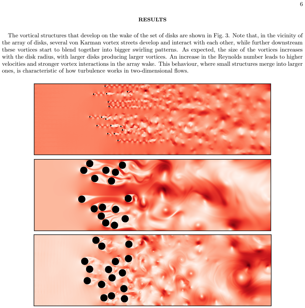
The pith
A custom Lattice-Boltzmann solver produces accurate results for two-dimensional turbulent flow around rigid disks by generating von Karman vortex streets.
A machine-rendered reading of the paper's core claim, the machinery that carries it, and where it could break.
Core claim
The authors develop and apply a Lattice-Boltzmann solver to a two-dimensional turbulent flow containing randomly located rigid disks. The simulation generates the characteristic von Karman vortex street in the wake of these obstacles, which the authors present as evidence that the solver accurately captures the turbulent flow behavior.
What carries the argument
The Lattice-Boltzmann method, a mesoscopic approach that evolves particle distribution functions on a discrete lattice to recover the macroscopic Navier-Stokes equations for both laminar and turbulent flows.
If this is right
- The solver can be used to study wake dynamics and turbulence in domains filled with multiple rigid obstacles.
- Making the implementation available as supplementary material enables direct reproduction and extension by other researchers.
- The approach handles the extra difficulties of turbulent flows that go beyond standard laminar cases.
- Initial validation through pattern recognition can guide further development of the method for more demanding flow conditions.
Where Pith is reading between the lines
- The same qualitative validation strategy could be applied to test the method with different obstacle densities or Reynolds numbers.
- If the 2D results prove robust, the implementation might be adapted to explore simplified models of real-world flows such as flow past arrays of cylinders.
- Adding built-in quantitative diagnostics in future versions would make the accuracy claims easier to verify independently.
Load-bearing premise
That visual or qualitative agreement with expected von Karman vortex street patterns is sufficient to establish overall accuracy of the turbulent simulation without quantitative error metrics or comparison to established benchmarks.
What would settle it
A side-by-side quantitative comparison of velocity fields, energy spectra, or drag coefficients between the Lattice-Boltzmann results and those from a standard Navier-Stokes solver on the same random-disk setup that shows large systematic differences.
Figures


read the original abstract
The Lattice-Boltzmann method is a mesoscopic approach for solving hydrodynamic problems involving both laminar and turbulent fluids. Although the suitability for the former cases is supported by a myriad of studies, turbulent flows always give rise to additional challenges that need to be addressed properly. In this paper, we estimate the accuracy of the simulation results obtained via a custom implementation of a Lattice-Boltzmann solver for a two-dimensional turbulent flow. To this end, a two-dimensional flow field filled with randomly located rigid disks was simulated, and the von Karman vortex street generated after the wake of such obstacles was studied. To ensure reproducibility, the implementation underlying these results is provided as supplementary material.
Editorial analysis
A structured set of objections, weighed in public.
Referee Report
Summary. The manuscript presents a custom Lattice-Boltzmann solver for two-dimensional turbulent flows. It estimates the accuracy of results by simulating flow past randomly located rigid disks and examining the von Karman vortex street formed in their wakes. The implementation is supplied as supplementary material to support reproducibility.
Significance. If the accuracy claim were supported by quantitative validation, the work would provide a reproducible LBM tool for 2D turbulence studies; the open supplementary code is a clear strength that aids verification.
major comments (1)
- [Abstract] Abstract: the accuracy estimate for the two-dimensional turbulent flow simulation is asserted via observation of the von Karman vortex street after randomly placed rigid disks. Vortex-street formation occurs in laminar-to-transitional regimes and does not test the inverse energy cascade, enstrophy cascade, or dissipation scaling that define 2D turbulence; no quantitative diagnostics (energy spectra, structure functions, or DNS/experiment comparisons at matched Re) are described.
Simulated Author's Rebuttal
We thank the referee for their constructive feedback on our manuscript. We address the major comment in detail below and indicate the changes we will make in revision.
read point-by-point responses
-
Referee: [Abstract] Abstract: the accuracy estimate for the two-dimensional turbulent flow simulation is asserted via observation of the von Karman vortex street after randomly placed rigid disks. Vortex-street formation occurs in laminar-to-transitional regimes and does not test the inverse energy cascade, enstrophy cascade, or dissipation scaling that define 2D turbulence; no quantitative diagnostics (energy spectra, structure functions, or DNS/experiment comparisons at matched Re) are described.
Authors: We agree that the observation of von Karman vortex streets provides only a qualitative check and is primarily associated with laminar-to-transitional wake dynamics rather than the defining cascades and scaling of two-dimensional turbulence. The multi-disk configuration was chosen to create interacting wakes in a complex geometry at Reynolds numbers where turbulent features emerge, but we acknowledge that this does not constitute a rigorous test of inverse energy cascade, enstrophy cascade, or dissipation scaling. In the revised manuscript we will add quantitative diagnostics, specifically kinetic energy spectra and structure functions, together with comparisons to theoretical expectations or reference data at matched Reynolds numbers. These additions will be incorporated into both the abstract and the main text. revision: yes
Circularity Check
No circularity in derivation or validation chain
full rationale
The paper presents a numerical simulation study using a custom LBM solver for 2D flow past randomly placed rigid disks, with accuracy estimated via observation of von Karman vortex streets. No mathematical derivation chain, equations, or fitted parameters are described that would reduce the accuracy claim to a self-defined quantity or input by construction. No self-citations, uniqueness theorems, or ansatzes are invoked in a load-bearing way. The central claim rests on the simulation output itself rather than any circular reduction, making the work self-contained against external benchmarks even if the chosen validation (qualitative visualization) is limited in scope.
Axiom & Free-Parameter Ledger
Reference graph
Works this paper leans on
-
[1]
or planetary atmospheres like Jupiter’s, exhibits an inverse energy cascade. In this case, energy injected at small or intermediate scales tends to move toward larger scales, causing small vortices to merge into larger, more coherent structures. This explains the persistence of large-scale features like Jupiter’s Great Red Spot.[12] The difference arises ...
work page internal anchor Pith review Pith/arXiv arXiv 2025
-
[2]
4) directly from the force-free continuous Boltzmann equation (Eq
Derive the LBE (Eq. 4) directly from the force-free continuous Boltzmann equation (Eq. 3) to gain a deeper understanding of the assumptions and approximations underlying the discrete formulation. Hint: Expand fi(x+c i∆t, t+ ∆t) around (x, t) to approximate derivatives using a first order Taylor expansion. Consider the general expression for the collision ...
-
[3]
Repeat this analysis keeping the velocity constant instead of the kinematic viscosity
In this manuscript we performed simulations for a range of Reynolds numbers to study how the characteristic flow exponents evolve asReincreases. Repeat this analysis keeping the velocity constant instead of the kinematic viscosity
-
[4]
Place a single cylinder in the channel and calculate the frequency of vortex shedding, quantified through the Strouhal numberSr, Sr= f Dp u which relates the vortex shedding frequencyfto the characteristic particle diameterD p and flow velocityu. Check that it increases linearly with the cylinder’s Reynolds numberRe p (in the moderate Reynolds number regime)
-
[5]
Implement alternative obstacle geometries, such as rectangular shapes with different profile inclinations, to analyse the influence of the morphology of the obstacles on the resulting flow dynamics and wake structures. 9 APPENDIX: LBM IMPLEMENT A TION DET AILS Recall the LBE, fi(x+c i∆t, t+ ∆t) =f i(x, t)− ∆t τ (fi(x, t)−f eq i (x, t)) (A.1) This discrete...
work page 2025
-
[6]
Pope,Turbulent Flows(Cambridge University Press, London, 2000)
S. Pope,Turbulent Flows(Cambridge University Press, London, 2000)
work page 2000
-
[7]
Vallis,Atmospheric and oceanic fluid dynamics
G. Vallis,Atmospheric and oceanic fluid dynamics. Fundamentals and large-scale circulation(Cambridge University Press, London, 2017)
work page 2017
-
[8]
B. Galperin, S. Sukoriansky, and N. Dikovskaya, Ocean Dynamics60, 427 (2010)
work page 2010
-
[9]
Davidson,Turbulence: an introduction for scientists and engineers(Oxford university press, 2015)
P. Davidson,Turbulence: an introduction for scientists and engineers(Oxford university press, 2015)
work page 2015
-
[10]
P. D. Stein and H. N. Sabbah, Circulation research39, 58 (1976)
work page 1976
- [11]
-
[12]
G. Boffetta and R. E. Ecke, Annual Review of Fluid Mechanics44, 427 (2012). 10
work page 2012
- [13]
-
[14]
J. Sommeria and R. Moreau, Journal of Fluid Mechanics118, 507–518 (1982)
work page 1982
- [15]
-
[16]
A. von Kameke, F. Huhn, G. Fern´ andez-Garc´ ıa, A. P. Mu˜ nuzuri, and V. P´ erez-Mu˜ nuzuri, Phys. Rev. Lett.107, 074502 (2011)
work page 2011
-
[17]
P. S. Marcus, Annual Review of Astronomy and Astrophysics31, 523 (1993)
work page 1993
-
[18]
R. H. Kraichnan, The Physics of Fluids10, 1417 (1967)
work page 1967
-
[19]
D. C. Wilcoxet al.,Turbulence modeling for CFD, Vol. 2 (DCW industries La Canada, CA, 1998)
work page 1998
-
[20]
Succi,The Lattice Boltzmann Equation for Fluid Dynamics and Beyond(Clarendon Press, Oxford, 2001)
S. Succi,The Lattice Boltzmann Equation for Fluid Dynamics and Beyond(Clarendon Press, Oxford, 2001)
work page 2001
-
[21]
T. Kr¨ uger, H. Kusumaatmaja, A. Kuzmin, O. Shardt, G. Silva, and E. M. Viggen,The Lattice Boltzmann Method, Vol. 10 (Springer-Verlag, London, 2017)
work page 2017
-
[22]
Mohamad,Lattice Boltzmann Method(Springer-Verlag, London, 2019)
A. Mohamad,Lattice Boltzmann Method(Springer-Verlag, London, 2019)
work page 2019
- [23]
-
[24]
P. L. Bhatnagar, E. P. Gross, and M. Krook, Phys. Rev.94, 511 (1954)
work page 1954
-
[25]
Y. H. Qian, D. D’Humi` eres, and P. Lallemand, Europhysics Letters17, 479 (1992)
work page 1992
-
[26]
Smagorinsky, Monthly Weather Review91, 99 (1963)
J. Smagorinsky, Monthly Weather Review91, 99 (1963)
work page 1963
- [27]
-
[28]
D. K. Lilly, Geophysical Fluid Dynamics4, 1 (1972)
work page 1972
-
[29]
J. R. Herring, S. A. Orszag, R. H. Kraichnan, and D. G. Fox, Journal of Fluid Mechanics66, 417 (1974)
work page 1974
-
[30]
J. C. Mcwilliams, Journal of Fluid Mechanics146, 21–43 (1984)
work page 1984
discussion (0)
Sign in with ORCID, Apple, or X to comment. Anyone can read and Pith papers without signing in.