A multiple-scales framework for branched channel filters
Pith reviewed 2026-05-18 00:33 UTC · model grok-4.3
The pith
Multiple-scales analysis produces an effective leakage boundary condition for flow over branched channel filters.
A machine-rendered reading of the paper's core claim, the machinery that carries it, and where it could break.
Core claim
We use multiple-scales techniques to derive an effective leakage boundary condition, which smooths out localised effects in the flow velocity and pressure that arise due to the discrete branched channels, and then use this boundary condition to explicitly determine the flow away from the boundary. We find that our explicit solution compares well with an analogous numerical solution containing a discrete set of branched channels. We further consider the behaviour of individual spherical particles in the device, with their trajectories determined via a simple force balance model with a wall-bounce condition, and explore the dependence of the fraction of particles that flow into the branched渠道s
What carries the argument
Effective leakage boundary condition obtained by multiple-scales averaging of discrete branched channels.
If this is right
- Velocity and pressure fields are available in closed form outside a thin layer near the filter surface.
- The smoothed boundary condition reproduces the far-field behavior of fully resolved discrete-channel computations.
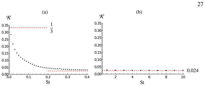
- Particle entry into branches is governed by Stokes number through the integrated trajectory equations.
- Overall filter efficiency becomes a direct function of branch spacing, flow speed, and particle properties.
Where Pith is reading between the lines
- The same averaging procedure could be applied to optimize branch angles or spacings for higher ricochet efficiency.
- Extensions to unsteady or lower-Reynolds-number regimes would require checking whether the scale separation still permits a simple leakage condition.
- The explicit flow solution offers a fast surrogate model for exploring parameter space before committing to detailed simulations.
Load-bearing premise
The separation between branches is much larger than the thickness of the viscous boundary layer.
What would settle it
A full numerical simulation of the discrete branched geometry that produces flow fields or particle-capture fractions differing substantially from the explicit multiple-scales solution.
Figures


read the original abstract
Fibres shed from our clothes during a washing machine cycle constitute around 35% of the primary microplastics in our oceans. Current conventional dead-end washing machine filters clog relatively quickly and require frequent cleaning. We consider a new concept, ricochet separation, inspired by the feeding process of manta rays, to reduce the cleaning frequency. In such a device, some fluid is diverted through branched channels whilst particles ricochet off the wall structure, forcing them back into the main flow and then into the dead-end filter. In this paper, we consider a simple branched-channel filter structure beneath a high-Reynolds-number laminar flow, in the case where the branch separation is much larger than the thickness of the viscous boundary layer. We use multiple-scales techniques to derive an effective leakage boundary condition, which smooths out localised effects in the flow velocity and pressure that arise due to the discrete branched channels, and then use this boundary condition to explicitly determine the flow away from the boundary. We find that our explicit solution compares well with an analogous numerical solution containing a discrete set of branched channels. We further consider the behaviour of individual spherical particles in the device, with their trajectories determined via a simple force balance model with a wall-bounce condition. We explore the dependence of the fraction of particles that flow into the branched channels on the particle's Stokes number. The resulting combined model is able to predict the relationship between the efficiency of a ricochet filter device and the design and operating parameters, avoiding the need to conduct extensive numerically challenging simulations.
Editorial analysis
A structured set of objections, weighed in public.
Referee Report
Summary. The paper develops a multiple-scales analysis for high-Reynolds-number laminar flow over a branched-channel filter where branch spacing greatly exceeds the viscous boundary-layer thickness. It derives an effective leakage boundary condition that homogenizes discrete-branch effects, obtains an explicit outer-flow solution, compares this solution to discrete-branch numerical simulations, and then uses a simple force-balance particle model with wall bounces to predict the fraction of particles entering the branches as a function of Stokes number, thereby relating device efficiency to design and operating parameters.
Significance. If the scale-separation assumption holds and the comparison is quantitatively sound, the work supplies a computationally inexpensive, parameter-free route to efficiency predictions that avoids full discrete simulations. The derivation from the governing equations under an explicit asymptotic assumption, together with the direct link to particle trajectories, constitutes a practical strength for microplastic-filter design.
major comments (2)
- [§4] §4 (numerical comparison): the claim that the explicit solution 'compares well' with the discrete-branch numerical solution is not accompanied by quantitative error measures (e.g., L2 or L∞ norms of velocity or pressure differences, or tabulated maximum relative errors). Without such metrics the support for the accuracy of the homogenized boundary condition remains qualitative and limits assessment of the approximation's robustness.
- [§5] §5 (particle trajectories): the dependence of branched-channel capture fraction on Stokes number is presented, yet the manuscript does not report the sensitivity of these curves to the wall-bounce restitution coefficient or to the precise form of the drag law; because the efficiency prediction rests on these trajectories, the lack of such checks weakens the quantitative reliability of the final design relations.
minor comments (2)
- [Figures 3–5] Figure captions and axis labels in the flow-field comparisons would benefit from explicit indication of which curves are analytic and which are numerical, together with a statement of the Reynolds number and branch-spacing ratio used.
- [Introduction] The introduction would be strengthened by a brief reference to prior multiple-scales treatments of perforated or ribbed walls to clarify the novelty of the leakage-condition derivation.
Simulated Author's Rebuttal
We thank the referee for their constructive review and recommendation of minor revision. We address each major comment below and will incorporate the suggested quantitative support in the revised manuscript.
read point-by-point responses
-
Referee: [§4] §4 (numerical comparison): the claim that the explicit solution 'compares well' with the discrete-branch numerical solution is not accompanied by quantitative error measures (e.g., L2 or L∞ norms of velocity or pressure differences, or tabulated maximum relative errors). Without such metrics the support for the accuracy of the homogenized boundary condition remains qualitative and limits assessment of the approximation's robustness.
Authors: We agree that quantitative error measures would strengthen the comparison. In the revised manuscript we will compute and report the L2 and L∞ norms of the velocity and pressure differences between the explicit multiple-scales solution and the discrete-branch numerical simulation. We will also tabulate maximum relative errors at representative locations along the boundary to provide a more rigorous quantification of the homogenized boundary condition's accuracy. revision: yes
-
Referee: [§5] §5 (particle trajectories): the dependence of branched-channel capture fraction on Stokes number is presented, yet the manuscript does not report the sensitivity of these curves to the wall-bounce restitution coefficient or to the precise form of the drag law; because the efficiency prediction rests on these trajectories, the lack of such checks weakens the quantitative reliability of the final design relations.
Authors: We acknowledge that the particle-capture results depend on modeling choices for bounces and drag. In the revised manuscript we will add a sensitivity study showing the capture-fraction curves for restitution coefficients between 0.7 and 1.0 and will compare the baseline Stokes-drag results with those obtained when an added-mass term is included. These additional checks will be presented to demonstrate that the reported Stokes-number dependence remains robust. revision: yes
Circularity Check
Multiple-scales derivation of effective leakage BC is self-contained asymptotic analysis
full rationale
The paper applies standard multiple-scales homogenization to the high-Re laminar flow equations under the explicit assumption that branch separation greatly exceeds viscous boundary-layer thickness. This produces an effective leakage boundary condition directly from the governing PDEs and scale-separation ansatz; the outer flow solution and subsequent particle trajectories follow from that BC without any parameter fitting to target data or renaming of known results. No self-citation chain, uniqueness theorem, or fitted-input-called-prediction appears in the derivation. The numerical comparison is performed inside the same asymptotic regime and serves as validation rather than input. The derivation chain therefore remains independent of its own outputs.
Axiom & Free-Parameter Ledger
axioms (2)
- domain assumption High-Reynolds-number laminar flow
- domain assumption Branch separation much larger than viscous boundary layer thickness
Reference graph
Works this paper leans on
-
[1]
ACHARYA, S., SHAIDA, S. R., YANG, H. & NOUREDDINE, A. 2021 Microfibers from synthetic textiles as a major source of microplastics in the environment: A review. Text. Res. J. 91 (17-18), 2136–2156. AKARSU, C., KUMBUR, H. & KIDEYS, A. E. 2021 Removal of microplastics from wastewater through electrocoagulation-electroflotation and membrane filtration process...
work page 2021
-
[2]
DIVI, R. V., STROTHER, J. A. & PAIG-TRAN, E. W. M. 2018 Manta rays feed using ricochet separation, a novel nonclogging filtration mechanism. Sci. Adv. 4 (9). DRIS, R., IMHOF, H. I., SANCHEZ, W. & GASPERI, J. 2015 Beyond the ocean: contamination of freshwater ecosystems with (micro-) plastic particles. Environ. Chem. 12 (5), 539–550. ENTEN, A. C., LEIPNER,...
work page 2018
-
[3]
HAMANN, L. 2023 Suspension feeders as biological models to develop biomimetic filter modules and reduce microplastic emissions. PhD thesis, Universitäts-und Landesbibliothek Bonn. HAZLEHURST, A., TIFFIN, L., SUMNER, M. & TAYLOR, M. 2023 Quantification of microfibre release from textiles during domestic laundering. Environ. Sci. Pollut. Res. 30 (15), 43932...
work page 2023
discussion (0)
Sign in with ORCID, Apple, or X to comment. Anyone can read and Pith papers without signing in.