Conditioning on posterior samples for flexible frequentist goodness-of-fit testing
Pith reviewed 2026-05-18 00:02 UTC · model grok-4.3
The pith
Conditioning on Bayesian posterior samples yields approximately valid frequentist goodness-of-fit tests for models without exact sufficient statistics.
A machine-rendered reading of the paper's core claim, the machinery that carries it, and where it could break.
Core claim
Samples from the posterior distribution of parameters given the data under the null serve as an approximate sufficient statistic. Conditioning on these samples generates artificial data sets that remain exchangeable with the observed data under the null. The resulting procedure, called approximately co-sufficient sampling via Bayes, produces an approximately valid p-value for any user-specified test statistic. The authors establish the approximate validity theoretically and illustrate practical gains on previously inaccessible models.
What carries the argument
approximately co-sufficient sampling via Bayes (aCSS-B), which treats posterior samples as an approximate sufficient statistic for generating exchangeable artificial data sets
If this is right
- The test maintains approximate validity for a broader class of null models than methods requiring exact sufficient statistics.
- Goodness-of-fit testing becomes feasible for three common null models with no prior applicable methods.
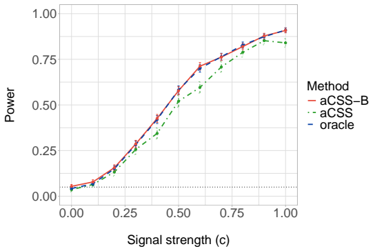
- On models where existing methods work, the new approach yields higher power.
- Analysts can apply any test statistic without sacrificing the approximate validity guarantee.
Where Pith is reading between the lines
- The technique could be combined with modern Bayesian sampling algorithms to handle high-dimensional or structured models.
- Similar posterior conditioning might extend to other frequentist procedures that rely on sufficient statistics, such as certain resampling methods.
- One could test the quality of the approximation by comparing posterior-based results to exact methods on models where both are feasible.
Load-bearing premise
The Bayesian posterior samples must be close enough to a true sufficient statistic that the test maintains approximate validity under the null.
What would settle it
Repeated simulations under a null model where the posterior is known to be a poor approximation to sufficiency would show the empirical type I error rate substantially exceeding the nominal level.
Figures


read the original abstract
Tests of goodness of fit are used in nearly every domain where statistics is applied. One powerful and flexible approach is to sample artificial data sets that are exchangeable with the real data under the null hypothesis (but not under the alternative), as this allows the analyst to conduct a valid test using any test statistic they desire. Such sampling is typically done by conditioning on either an exact or approximate sufficient statistic, but existing methods for doing so have significant limitations, which either preclude their use or substantially reduce their power or computational tractability for many important models. In this paper, we propose to condition on samples from a Bayesian posterior distribution, which constitute a very different type of approximate sufficient statistic than those considered in prior work. Our approach, approximately co-sufficient sampling via Bayes (aCSS-B), considerably expands the scope of this flexible type of goodness-of-fit testing. We prove the approximate validity of the resulting test, and demonstrate its utility on three common null models where no existing methods apply, as well as its outperformance on models where existing methods do apply.
Editorial analysis
A structured set of objections, weighed in public.
Referee Report
Summary. The manuscript proposes approximately co-sufficient sampling via Bayes (aCSS-B), which generates artificial data for goodness-of-fit testing by conditioning on draws from a Bayesian posterior distribution rather than an exact or previously studied approximate sufficient statistic. The authors assert a proof of approximate validity for the resulting test and provide empirical demonstrations on three common null models where no existing methods apply, together with outperformance results on models where prior methods exist.
Significance. If the approximate validity holds with explicit, verifiable error bounds that remain controlled for the targeted models, the method would meaningfully enlarge the class of models for which flexible, user-specified test statistics can be used in frequentist GOF testing while retaining approximate type-I error control.
major comments (2)
- [Theoretical results section (following method definition)] Proof of approximate validity: the manuscript states that a proof is given, yet supplies no explicit bound (e.g., in total variation or Kolmogorov distance) relating the posterior approximation error to the deviation of the p-value from uniformity under the null. This translation step is load-bearing for the central claim that the procedure remains approximately valid for the three models where existing methods fail; without a rate or dependence on prior choice and posterior concentration, the scope-expansion claim cannot be verified from the given derivation.
- [Numerical experiments section] Application to the three null models: the empirical demonstrations do not include a quantitative check that the posterior-to-sufficient-statistic distance is small enough under the chosen priors and sample sizes to keep type-I error inflation below a stated tolerance. This is required to substantiate that the method succeeds precisely where prior co-sufficient approaches do not apply.
minor comments (2)
- [Method description] Notation for the artificial data generation step could be clarified to distinguish the posterior draw from the exact sufficient statistic more explicitly.
- [Abstract] The abstract would benefit from a single sentence stating the main regularity conditions under which the approximate validity holds.
Simulated Author's Rebuttal
We thank the referee for their constructive and detailed comments, which highlight important opportunities to strengthen the explicitness of our theoretical guarantees and the quantitative validation of our empirical results. We address each major comment below and will incorporate the suggested clarifications in a revised manuscript.
read point-by-point responses
-
Referee: [Theoretical results section (following method definition)] Proof of approximate validity: the manuscript states that a proof is given, yet supplies no explicit bound (e.g., in total variation or Kolmogorov distance) relating the posterior approximation error to the deviation of the p-value from uniformity under the null. This translation step is load-bearing for the central claim that the procedure remains approximately valid for the three models where existing methods fail; without a rate or dependence on prior choice and posterior concentration, the scope-expansion claim cannot be verified from the given derivation.
Authors: We agree that the current presentation of the proof could be strengthened by making the error translation more explicit. The existing argument bounds the total variation distance between the law of the test statistic conditional on a posterior draw and the law conditional on an exact sufficient statistic, then invokes this to control the deviation of the p-value from uniformity. However, we acknowledge that explicit rates linking this distance to posterior approximation error, prior choice, and concentration are not stated as a corollary. In revision we will add a new corollary that supplies such a bound (in total variation) together with a brief discussion of its dependence on the prior and sample size for the three targeted models. This will make the scope-expansion claim directly verifiable from the derivation. revision: yes
-
Referee: [Numerical experiments section] Application to the three null models: the empirical demonstrations do not include a quantitative check that the posterior-to-sufficient-statistic distance is small enough under the chosen priors and sample sizes to keep type-I error inflation below a stated tolerance. This is required to substantiate that the method succeeds precisely where prior co-sufficient approaches do not apply.
Authors: The referee correctly identifies that our simulations show type-I error rates close to nominal levels but do not report a direct quantitative metric of the posterior-to-sufficient-statistic distance. We will revise the numerical experiments section to include such checks—for instance, by computing and reporting the average total variation (or Wasserstein) distance between posterior samples and the true (or best available) sufficient statistic across Monte Carlo replications, and by relating these distances to the observed type-I error inflation for each model and sample size. This addition will provide the requested substantiation that the approximation quality is sufficient for the models where existing methods do not apply. revision: yes
Circularity Check
No significant circularity; derivation is self-contained
full rationale
The paper introduces aCSS-B by conditioning on Bayesian posterior samples as an approximate sufficient statistic for flexible goodness-of-fit testing. It claims a proof of approximate validity and demonstrates the method on three null models. No equations or steps in the abstract or described content reduce a claimed prediction or validity result to a fitted parameter or self-citation by construction. The posterior sampling step is external to the frequentist test construction and does not rely on self-definitional loops, fitted inputs renamed as predictions, or load-bearing self-citations that collapse the central claim. The derivation therefore remains independent of its own outputs.
Axiom & Free-Parameter Ledger
axioms (1)
- domain assumption Posterior samples from a Bayesian model provide an approximate sufficient statistic for the null distribution in the sense required for co-sufficient sampling.
Lean theorems connected to this paper
-
IndisputableMonolith/Cost/FunctionalEquation.leanwashburn_uniqueness_aczel unclear?
unclearRelation between the paper passage and the cited Recognition theorem.
We propose to condition on samples from a Bayesian posterior distribution... prove the approximate validity of the resulting test
-
IndisputableMonolith/Foundation/RealityFromDistinction.leanreality_from_one_distinction unclear?
unclearRelation between the paper passage and the cited Recognition theorem.
Theorem 3.1... dexch(X, eX(1), …, eX(M)) ≤ inf_π0 {ϵ(π0) + Δ(π0)/(2√B)}
What do these tags mean?
- matches
- The paper's claim is directly supported by a theorem in the formal canon.
- supports
- The theorem supports part of the paper's argument, but the paper may add assumptions or extra steps.
- extends
- The paper goes beyond the formal theorem; the theorem is a base layer rather than the whole result.
- uses
- The paper appears to rely on the theorem as machinery.
- contradicts
- The paper's claim conflicts with a theorem or certificate in the canon.
- unclear
- Pith found a possible connection, but the passage is too broad, indirect, or ambiguous to say the theorem truly supports the claim.
Reference graph
Works this paper leans on
-
[1]
= wj ϕ(xi;µ j, σ2 j ) P2 ℓ=1 wℓ ϕ(xi;µ ℓ, σ2 ℓ ) , i= 1, . . . , n,(24) w1 |Z∼Beta (2 +n 1,2 +n 2), n j = nX i=1 1{Zi =j},(25) µj |σ 2 j , Z, X∼ N P i:zi=j xi 1 +n j , σ2 j 1 +n j ,(26) σ2 j |µ j, Z, X∼Inv-Gamma 3 2 + nj 2 , 1 2 + 1 2 X i:Zi=j (xi −µ j)2 + 1 2 µ2 j ! .(27) These allow for efficient sampling using the Gibbs sampler. We begin by initializin...
-
[2]
Independently for eachi, sample eachZ (t) i |X, w (t−1), µ (t−1), σ 2,(t−1) according to (24)
-
[3]
Samplew (t) 1 Z(t) according to (25), and setw (t) 2 = 1−w (t) 1
-
[4]
4n2/2 (2π)n2/2 (1 + 4∥V∥ 2 2)n/2 e −2∥x∥2 F+8 ∥diag{d}V∥ 2 2 1+4∥V∥ 2 2 # =E W1,...,Wn iid∼χ 2 1
For eachj= 1,2, drawµ (t) j |σ 2,(t−1) j , Z(t), Xandσ 2,(t) j |µ (t) j , Z(t), Xaccording to (26) and (27), respectively. We discard the first 500 draws and extract the posterior samples bθ1, . . . ,bθB at every tenth step. Sampling the copies:To sample the copies, we again use an approximation of the marginal ¯fπ(x) and sample from bgπ(x| bθ1:B)∝ QB b=1...
work page 2023
-
[5]
Generateγ (b) fromγ|t (b−1) 1 , Z, Xas in Equation (31)
-
[6]
After the burn-in ofB 0 = 500, we extractB= 25 posterior samples{t (b), γ(b)}at every tenth step
Generatet (b) 1 fromt 1 |Z, X, γ (b) as in Equation (34). After the burn-in ofB 0 = 500, we extractB= 25 posterior samples{t (b), γ(b)}at every tenth step. Sampling the copies:Our first step is to approximate the marginal ¯fπ(x). In this case, we first marginalize outγfrom the distribution ofX|t, γas follows: X|t 1, γ∼ N(h t(Z)γ,0.25I n) =⇒X|t 1 ∼ N 0n, h...
discussion (0)
Sign in with ORCID, Apple, or X to comment. Anyone can read and Pith papers without signing in.