arxiv: 2512.17038 · v3 · submitted 2025-12-18 · 📊 stat.AP

Do Generalized-Gamma Scale Mixtures of Normals Fit Large Image Datasets?

Brandon Marks , Yash Dave , Zixun Wang , Hannah Chung , Riya Patwa , Simon Cha , Michael Murphy , Alexander Strang This is my paper

Pith reviewed 2026-05-16 20:50 UTC · model grok-4.3

classification 📊 stat.AP

keywords generalized gamma distributionscale mixture of normalsimage priorsBayesian inferencewavelet transformsFourier transformsconvolutional neural networksremote sensing

0 comments p. Extension

The pith

Generalized gamma scale mixtures of normals fit image coefficients from remote sensing, medical, and classification datasets better than Gaussian, Laplace, or Student-t priors.

A machine-rendered reading of the paper's core claim, the machinery that carries it, and where it could break.

The paper examines whether generalized gamma scale mixtures of normals act as realistic priors for large collections of image data. It applies the model to Fourier transforms, Haar and Gabor wavelets, and coefficients from the first layer of a trained convolutional network across remote sensing, medical imaging, and classification images. Data-augmentation steps and selection of exchangeable coefficients improve the observed fit. The two-parameter family outperforms the standard distributions it contains, including Gaussian, Laplace, ell-p, and t distributions, over broad parameter regions. The work also flags image features that cause the model to fit poorly.

Core claim

Generalized-gamma scale mixtures of normals are realistic for multiple large imaging data sets drawn from remote sensing, medical imaging, and image classification applications when applied to Fourier and wavelet transformations of the images as well as to coefficients produced by convolving against AlexNet first-layer filters, and this prior family provides a substantially better fit to each data set than Gaussian, Laplace, ell-p, or Student's t priors.

What carries the argument

The generalized gamma scale mixture of normals, formed by mixing normals of fixed mean with variances drawn from a generalized gamma distribution whose two shape parameters separately control behavior near the mode and tail decay.

If this is right

The prior can be used with greater confidence in Bayesian formulations of inverse imaging problems.
Parameter regions substantially broader than those emphasized in earlier computational work describe the observed data.
Data-augmentation procedures and exchangeability screening are required to achieve the reported fit quality.
The model remains unrealistic for images whose characteristic features produce heavy selection effects or non-exchangeable coefficients.

Where Pith is reading between the lines

These are editorial extensions of the paper, not claims the author makes directly.

The same prior family could be tested on coefficients from deeper layers of convolutional networks or on other high-dimensional signals such as audio spectrograms.
Identifying the specific image features that cause poor fit may guide the design of hybrid priors that switch between families depending on local image statistics.
If the exchangeability assumption holds more generally, the two shape parameters could be estimated once from a representative image corpus and then reused across related inverse problems.

Load-bearing premise

Data-augmentation procedures produce approximately exchangeable coefficients whose marginal distribution can be treated as i.i.d. draws from the generalized-gamma scale mixture without selection bias that inflates apparent fit quality.

What would settle it

A large image dataset, after the same augmentation and exchangeability filtering, where the generalized gamma mixture yields a worse or equal fit to the data compared with Gaussian, Laplace, ell-p, or t priors.

Figures

Figures reproduced from arXiv: 2512.17038 by Alexander Strang, Brandon Marks, Hannah Chung, Michael Murphy, Riya Patwa, Simon Cha, Yash Dave, Zixun Wang.

**Figure 1.** Figure 1: Each layer of the stacked plot is a normal distribution with mean 0 and variance drawn from a generalized [PITH_FULL_IMAGE:figures/full_fig_p004_1.png] view at source ↗

**Figure 2.** Figure 2: Parameter space map with commonly used priors (Cauchy, Student’s [PITH_FULL_IMAGE:figures/full_fig_p005_2.png] view at source ↗

**Figure 3.** Figure 3: Sensitivity of the prior to perturbations in the shape parameters [PITH_FULL_IMAGE:figures/full_fig_p006_3.png] view at source ↗

**Figure 4.** Figure 4: Changes in the scale parameter ϑ can be used to compensate for changes in r and η. The red and black curves differ in their tail decay rates and smoothness of their peaks. Decreasing ϑ bridges this gap, with ϑ = 0.075 producing approximately the same distribution. The log-density plot shows that the tails are slightly smaller for the blue curve, but the peak of the distribution is a near-perfect match. Adj… view at source ↗

**Figure 5.** Figure 5: Representative sample(s) from each of the remote sensing, natural, medical, and classical image datasets. [PITH_FULL_IMAGE:figures/full_fig_p009_5.png] view at source ↗

**Figure 6.** Figure 6: Example of Haar wavelet transform applied to the MIT cameraman image, ordered from low (Layer 5) to high [PITH_FULL_IMAGE:figures/full_fig_p011_6.png] view at source ↗

**Figure 7.** Figure 7: Visualization of representative filter from each filter group, normalized 0-1, from the first layer of AlexNet. See [PITH_FULL_IMAGE:figures/full_fig_p012_7.png] view at source ↗

**Figure 8.** Figure 8: Data augmentation model used to justify exchangeability. The solid green arrows represent the workflow [PITH_FULL_IMAGE:figures/full_fig_p013_8.png] view at source ↗

**Figure 9.** Figure 9: Process for grouping coefficients into ”bands” after applying a Fourier transform, as described in [PITH_FULL_IMAGE:figures/full_fig_p014_9.png] view at source ↗

**Figure 10.** Figure 10: Two high-quality fits to distributions with different peak and tail behavior. The top row (pastis, Fourier, gray, [PITH_FULL_IMAGE:figures/full_fig_p017_10.png] view at source ↗

**Figure 11.** Figure 11: KS statistics organized by transform and dataset type, colored by dataset. The horizontal position of each point [PITH_FULL_IMAGE:figures/full_fig_p018_11.png] view at source ↗

**Figure 12.** Figure 12: KS statistics for select dataset-transform combinations with the remote sensing datasets ( [PITH_FULL_IMAGE:figures/full_fig_p020_12.png] view at source ↗

**Figure 13.** Figure 13: KS statistics for select dataset-transform combinations with the natural image datasets ( [PITH_FULL_IMAGE:figures/full_fig_p020_13.png] view at source ↗

**Figure 14.** Figure 14: KS statistics for select dataset-transform combinations with the medical image datasets ( [PITH_FULL_IMAGE:figures/full_fig_p021_14.png] view at source ↗

**Figure 15.** Figure 15: KS statistics for the remote sensing and natural image datasets after applying the learned filters, aggregating [PITH_FULL_IMAGE:figures/full_fig_p021_15.png] view at source ↗

**Figure 16.** Figure 16: Best fit parameters categorized by fit category (see Table [PITH_FULL_IMAGE:figures/full_fig_p022_16.png] view at source ↗

**Figure 17.** Figure 17: Two similar fits to a sample (agriVision, Wavelet Diagonal, Layer 6) after picking the scale parameter by [PITH_FULL_IMAGE:figures/full_fig_p025_17.png] view at source ↗

**Figure 18.** Figure 18: Visualization of all 64 learned filters used, normalized 0-1, from the first layer of AlexNet with their filter [PITH_FULL_IMAGE:figures/full_fig_p030_18.png] view at source ↗

**Figure 19.** Figure 19: This plot shows representative fit categorizations from all the non-trivial failure categories. The parameters [PITH_FULL_IMAGE:figures/full_fig_p032_19.png] view at source ↗

**Figure 20.** Figure 20: This plot shows representative fit categorizations from all the trivial failure subcategories. The parameters for [PITH_FULL_IMAGE:figures/full_fig_p033_20.png] view at source ↗

**Figure 21.** Figure 21: The blue shaded region shows the area being integrated over equations ( [PITH_FULL_IMAGE:figures/full_fig_p034_21.png] view at source ↗

read the original abstract

A scale mixture of normals is a distribution formed by mixing a collection of normal distributions with fixed mean but different variances. A generalized gamma scale mixture draws the variances from a generalized gamma distribution. Generalized gamma scale mixtures of normals have been proposed as an attractive class of parametric priors for Bayesian inference in inverse imaging problems. Generalized gamma scale mixtures have two shape parameters, one that controls the behavior of the distribution about its mode, and the other that controls its tail decay. In this paper, we provide the first demonstration that the prior model is realistic for multiple large imaging data sets. We draw data from remote sensing, medical imaging, and image classification applications. We study the realism of the prior when applied to Fourier and wavelet (Haar and Gabor) transformations of the images, as well as to the coefficients produced by convolving the images against the filters used in the first layer of AlexNet, a popular convolutional neural network trained for image classification. We discuss data augmentation procedures that improve the fit of the model, procedures for identifying approximately exchangeable coefficients, and characterize the parameter regions that best describe the observed data sets. These regions are significantly broader than the region of primary focus in computational work. We show that this prior family provides a substantially better fit to each data set than any of the standard priors it contains. These include Gaussian, Laplace, $\ell_p$, and Student's $t$ priors. Finally, we identify cases where the prior is unrealistic and highlight characteristic features of images that suggest the model will fit poorly.

Editorial analysis

A structured set of objections, weighed in public.

Desk editor's note, referee report, simulated authors' rebuttal, and a circularity audit. Tearing a paper down is the easy half of reading it; the pith above is the substance, this is the friction.

Desk Editor's Note private letter to a colleague

The paper shows generalized-gamma scale mixtures fit image coefficients better than standard priors across several large datasets, but the gains depend on augmentation and selection steps whose bias risk is not quantified.

read the letter

The core finding is that generalized-gamma scale mixtures of normals match the marginals of Fourier, wavelet, and AlexNet first-layer coefficients from remote-sensing, medical, and classification images better than Gaussian, Laplace, or t priors. They map the two shape parameters that work across these domains and note where the model breaks down, which is the first time this has been checked at this scale on real data rather than synthetic examples. That breadth and the parameter characterization are the useful parts; they give practitioners a concrete sense of when the prior is plausible and when it is not. The practical discussion of augmentation to improve fit and rules for picking approximately exchangeable coefficients also shows they thought about how to apply the model to messy image data. The soft spot is exactly the one the stress test flags. The abstract says augmentation and exchangeability procedures are used to improve the fit, yet supplies no numbers on how much data is discarded, no sensitivity checks, and no downstream validation on inverse-problem performance. Without those, it is hard to tell whether the reported superiority is a property of typical image coefficients or an artifact of the preprocessing pipeline that preferentially keeps samples the two-parameter family can describe. The lack of any goodness-of-fit statistics, cross-validation, or error bars in the abstract makes the evidence look thinner than the claim requires. This is the kind of paper that belongs in a reading group focused on priors for imaging. Readers working on Bayesian inverse problems would get concrete guidance on parameter ranges and failure modes. It is worth sending to peer review because the empirical scope is real and the model class is already in use; referees will need to press on the data-handling steps and ask for quantitative fit measures and predictive checks, but the work is coherent enough to deserve that scrutiny rather than a desk reject.

Referee Report

2 major / 2 minor

Summary. The paper empirically tests whether generalized-gamma scale mixtures of normals (with two shape parameters controlling mode behavior and tail decay) provide realistic priors for coefficients arising from Fourier, wavelet (Haar/Gabor), and AlexNet first-layer transformations of large image datasets drawn from remote sensing, medical imaging, and classification tasks. It introduces data-augmentation procedures and methods to select approximately exchangeable coefficients, characterizes the best-fitting parameter regions (broader than those emphasized in prior computational work), and claims that this two-parameter family yields substantially better fits than the Gaussian, Laplace, ℓ_p, and Student-t special cases it contains. The work also flags image features where the model fits poorly.

Significance. If the reported superior fits survive scrutiny for preprocessing bias, the result would supply the first large-scale empirical validation that generalized-gamma scale mixtures are realistic for real imaging coefficients. This would strengthen the case for using this prior family in Bayesian inverse problems, where the extra flexibility over standard heavy-tailed choices could improve reconstruction quality. The identification of broader parameter regions and failure modes would also guide practical prior selection.

major comments (2)

[Methods (data augmentation and exchangeability)] Methods section on data augmentation and exchangeability identification: the central claim that the prior family fits substantially better than its special cases rests on the assumption that augmentation and exchangeability selection produce approximately i.i.d. draws without preferentially retaining samples whose marginals match the two-parameter family. No comparison of fits before versus after selection, nor predictive checks on held-out images, is described that would rule out selection bias inflating the reported superiority.
[Results] Results section (quantitative fit comparisons): the abstract asserts substantially better fits but supplies no numerical goodness-of-fit statistics (e.g., log-likelihood ratios, Kolmogorov-Smirnov distances, or cross-validated predictive scores) with error bars or details on post-hoc exclusions. Without these, it is impossible to assess whether the improvement is statistically meaningful or driven by fitting choices.

minor comments (2)

[Methods] Clarify the precise definition of 'approximately exchangeable' and the quantitative criterion used to retain coefficients; this notation appears without an explicit threshold or algorithm in the abstract.
[Figures] Figure captions should report the exact number of coefficients retained after exchangeability filtering for each dataset and transformation, to allow readers to gauge sample size.

Simulated Author's Rebuttal

2 responses · 0 unresolved

We thank the referee for the constructive and detailed comments, which have prompted us to strengthen the empirical support in the manuscript. We address each major comment below and have revised the paper accordingly.

read point-by-point responses

Referee: [Methods (data augmentation and exchangeability)] Methods section on data augmentation and exchangeability identification: the central claim that the prior family fits substantially better than its special cases rests on the assumption that augmentation and exchangeability selection produce approximately i.i.d. draws without preferentially retaining samples whose marginals match the two-parameter family. No comparison of fits before versus after selection, nor predictive checks on held-out images, is described that would rule out selection bias inflating the reported superiority.

Authors: We agree that the absence of explicit before-versus-after comparisons leaves open the possibility of selection bias. In the revised manuscript we will add direct quantitative comparisons of goodness-of-fit (log-likelihood and Kolmogorov-Smirnov statistics) on the raw coefficient sets versus the post-augmentation, post-exchangeability-selected sets. We will also include posterior predictive checks on held-out images drawn from each application domain to confirm that the reported superiority is not an artifact of the selection procedure. revision: yes
Referee: [Results] Results section (quantitative fit comparisons): the abstract asserts substantially better fits but supplies no numerical goodness-of-fit statistics (e.g., log-likelihood ratios, Kolmogorov-Smirnov distances, or cross-validated predictive scores) with error bars or details on post-hoc exclusions. Without these, it is impossible to assess whether the improvement is statistically meaningful or driven by fitting choices.

Authors: We accept that the current version lacks the numerical summaries needed for rigorous evaluation. The revised manuscript will report log-likelihood ratios (with bootstrap standard errors), Kolmogorov-Smirnov distances, and cross-validated predictive scores for the generalized-gamma scale mixture versus each of its special cases, together with an explicit account of any post-hoc exclusions. These additions will allow readers to judge both the magnitude and statistical significance of the reported improvements. revision: yes

Circularity Check

0 steps flagged

No circularity: empirical marginal fits to image coefficients

full rationale

The paper performs direct empirical comparisons by fitting the two-parameter generalized-gamma scale mixture to observed histograms of Fourier, wavelet, and AlexNet coefficients drawn from multiple large imaging datasets. No derivation, prediction, or uniqueness claim is advanced that reduces by construction to a quantity defined from the fitted parameters themselves. The reported superiority over the one-parameter special cases (Gaussian, Laplace, Student-t) follows from standard likelihood or goodness-of-fit comparison on the same data; the extra flexibility is explicit and the paper also identifies regimes where the model fits poorly. Data-augmentation and exchangeability-selection steps are preprocessing choices whose effect on apparent fit quality can be checked against held-out coefficients or alternative transforms; they do not create a self-referential loop inside any equation. No self-citation supplies a load-bearing uniqueness theorem or ansatz. The analysis is therefore self-contained against external data benchmarks.

Axiom & Free-Parameter Ledger

1 free parameters · 1 axioms · 0 invented entities

The central claim rests on the assumption that transformed image coefficients can be grouped into approximately exchangeable sets via data augmentation and that the generalized-gamma scale mixture is an adequate marginal model for those sets. No new physical entities are introduced; the two shape parameters are fitted to data.

free parameters (1)

two shape parameters of generalized gamma
Control peak behavior and tail decay; fitted to each dataset's coefficient histograms.

axioms (1)

domain assumption Transformed coefficients are approximately exchangeable after data augmentation
Invoked when the authors discuss procedures for identifying exchangeable coefficients and when they pool data across images.

pith-pipeline@v0.9.0 · 5589 in / 1311 out tokens · 24442 ms · 2026-05-16T20:50:21.483890+00:00 · methodology

discussion (0)

Lean theorems connected to this paper

Citations machine-checked in the Pith Canon. Every link opens the source theorem in the public Lean library.

IndisputableMonolith/Cost/FunctionalEquation.lean washburn_uniqueness_aczel unclear

?

unclear
Relation between the paper passage and the cited Recognition theorem.

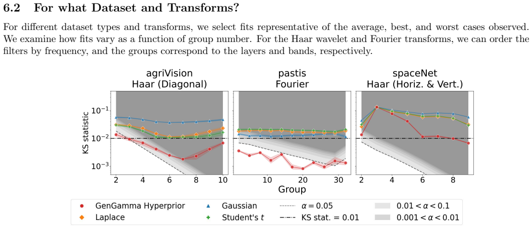
We show that this prior family provides a substantially better fit to each data set than any of the standard priors it contains. These include Gaussian, Laplace, ℓp, and Student’s t priors.
IndisputableMonolith/Foundation/Atomicity.lean atomic_tick unclear

?

unclear
Relation between the paper passage and the cited Recognition theorem.

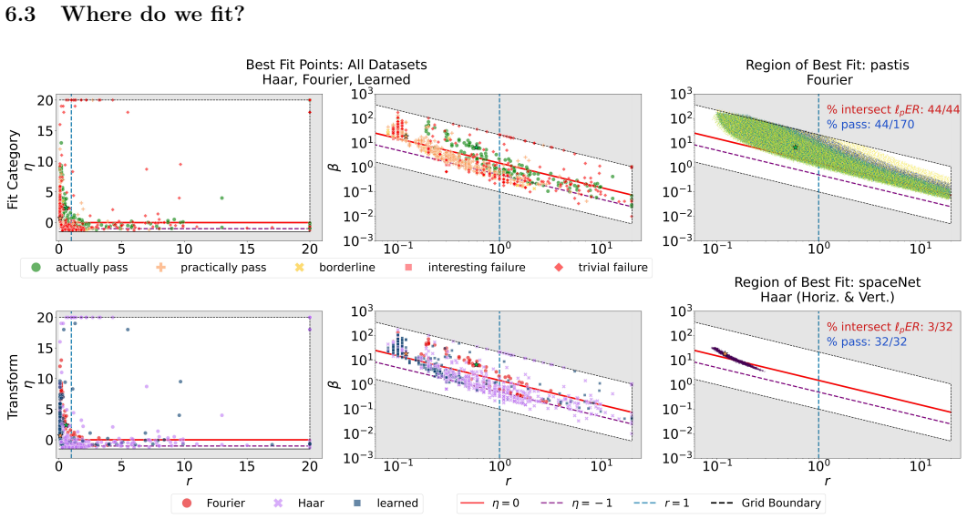
We discuss data augmentation procedures that improve the fit of the model, procedures for identifying approximately exchangeable coefficients

What do these tags mean?

matches: The paper's claim is directly supported by a theorem in the formal canon.
supports: The theorem supports part of the paper's argument, but the paper may add assumptions or extra steps.
extends: The paper goes beyond the formal theorem; the theorem is a base layer rather than the whole result.
uses: The paper appears to rely on the theorem as machinery.
contradicts: The paper's claim conflicts with a theorem or certificate in the canon.
unclear: Pith found a possible connection, but the passage is too broad, indirect, or ambiguous to say the theorem truly supports the claim.

Reference graph

Works this paper leans on

28 extracted references · 28 canonical work pages

[1]

Abanto-Valle, D

[1]C. Abanto-Valle, D. Bandyopadhyay, V. Lachos, and I. Enriquez, Robust bayesian analysis of heavy-tailed stochastic volatility models using scale mixtures of normal distributions, Computational Statistics & Data Analysis, 54 (2010), pp. 2883–2898. [2]S. Agrawal, H. Kim, D. Sanz-Alonso, and A. Strang, A variational inference approach to inverse problems ...

work page 2010
[2]

[5]S. D. Babacan, R. Molina, and A. K. Katsaggelos, Bayesian compressive sensing using laplace priors, IEEE Transactions on Image Processing, 19 (2010), pp. 53–63. [6]S. Bhadra, W. Zhou, and M. A. Anastasio, Medical image reconstruction with image-adaptive priors learned by use of generative adversarial networks,

work page 2010
[3]

Buades, B

[7]A. Buades, B. Coll, and J. M. Morel, A review of image denoising algorithms, with a new one, Multiscale Modeling & Simulation, 4 (2005), pp. 490–530. [8]D. Calvetti, R. K. Dash, E. Somersalo, and M. E. Cabrera, Local regularization method applied to estimating oxygen consumption during muscle activities, Inverse Problems, 22 (2006), pp. 229– 243.https:...

work page doi:10.1088/0266-5611/22/1/013 2005
[4]

, Brain activity mapping from MEG data via a hierarchical Bayesian algorithm with automatic depth weighting, Brain topography, 32 (2019), pp. 363–393. [12]D. Calvetti, F. Pitolli, E. Somersalo, and B. Vantaggi, Bayes meets Krylov: Statistically inspired preconditioners for CGLS, SIAM Review, 60 (2018), pp. 429–461. [13]D. Calvetti, M. Pragliola, and E. So...

work page 2019
[5]

Dong and M

26 [23]Y. Dong and M. Pragliola, Inducing sparsity via the horseshoe prior in imaging problems, Inverse Problems, 39 (2023), p. 074001. [24]D. L. Donoho, M. Elad, and V. N. Temlyakov, Stable recovery of sparse overcomplete representations in the presence of noise, IEEE Transactions on information theory, 52 (2005), pp. 6–18. [25]M. A. Figueiredo, R. D. No...

work page 2023
[6]

Glaubitz and A

[28]J. Glaubitz and A. Gelb, Leveraging joint sparsity in hierarchical bayesian learning, SIAM/ASA Journal on Uncertainty Quantification, 12 (2024), pp. 442–472. [29]J. Glaubitz, A. Gelb, and G. Song, Generalized sparse bayesian learning and application to image reconstruction, SIAM/ASA Journal on Uncertainty Quantification, 11 (2023), p. 262–284. [30]J. ...

work page arXiv 2024
[7]

Lindbloom, J

[38]J. Lindbloom, J. Glaubitz, and A. Gelb, Efficient sparsity-promoting map estimation for bayesian linear inverse problems, Inverse Problems, 41 (2025), p. 025001. [39]A. Manninen, M. Mozumder, T. Tarvainen, and A. Hauptmann, Sparsity promoting reconstructions via hierarchical prior models in diffuse optical tomography, Inverse Problems and Imaging, 18 ...

work page 2025
[8]

Pragliola, D

[46]M. Pragliola, D. Calvetti, and E. Somersalo, Overcomplete representation in a hierarchical Bayesian framework, arXiv preprint arXiv:2006.13524, (2020). [47]L. Roininen, M. Girolami, S. Lasanen, and M. Markkanen, Hyperpriors for mat´ ernfields with applications in bayesian inversion, Inverse Problems and Imaging, 13 (2019), pp. 1–29. [48]J. Shermeyer, ...

work page arXiv 2006
[9]

[49]Z. Si, Y. Liu, and A. Strang, Path-following methods for maximum a posteriori estimators in bayesian hierarchical models: How estimates depend on hyperparameters, SIAM Journal on Optimization, 34 (2024), pp. 2201–2230. [50]J. Suuronen, N. K. Chada, and L. Roininen, Cauchy markov random field priors for bayesian inversion, Statistics and Computing, 32 ...

work page arXiv 2024
[10]

Xiao and J

[54]Y. Xiao and J. Glaubitz, Sequential image recovery using joint hierarchical bayesian learning, Journal of Scientific Computing, 96 (2023). [55]H. Zou and T. Hastie, Regularization and variable selection via the elastic net, Journal of the Royal Statistical Society Series B: Statistical Methodology, 67 (2005), pp. 301–320. 28 A Survey of Computational ...

work page 2023
[11]

2008 Computed / Synthetic Computational Conditionally Gaussian hypermodels for cerebral source local- ization

work page 2008
[12]

2009 Computed / Synthetic Application Sparse Bayesian image Restoration

work page 2009
[13]

2010 Classic Application A hierarchical Krylov–Bayes iterative inverse solver for MEG with physiological preconditioning

work page 2010
[14]

2015 Computed / Synthetic Application Bayes meets Krylov: Statistically inspired preconditioners for CGLS

work page 2015
[15]

2018 Computed / Synthetic Computational Brain activity mapping from MEG data via a hierarchical Bayesian algorithm with automatic depth weighting

work page 2018
[16]

2019 Real and Synthetic Application Hierarchical Bayesian models and sparsity:ℓ 2-magic

work page 2019
[17]

2019 Computed / Synthetic Computational Sparse reconstructions from few noisy data: analysis of hier- archical Bayesian models with generalized gamma hyperpriors

work page 2019
[18]

2020 Computed / Synthetic Computational Sparsity promoting hybrid solvers for hierarchical Bayesian in- verse problems

work page 2020
[19]

2020 Computed / Synthetic Computational Overcomplete representation in a hierarchical Bayesian frame- work

work page 2020
[20]

2020 Computed / Synthetic Computational A variational inference approach to inverse problems with gamma hyperpriors

work page 2020
[21]

2022 Computed / Synthetic Computational Hierarchical ensemble Kalman methods with sparsity-promoting generalized Gamma hyperpriors

work page 2022
[22]

2022 Computed / Synthetic Computational Hierarchical Ensemble Kalman Methods with Sparsity- Promoting Generalized Gamma Hyperpriors

work page 2022
[23]

2022 Computed / Synthetic Computational Sparsity promoting reconstructions via hierarchical prior mod- els in diffuse optical tomography

work page 2022
[24]

2023 Computed / Synthetic Computational Sequential image recovery using joint hierarchical Bayesian learning

work page 2023
[25]

2023 Real and Synthetic Computational Leveraging joint sparsity in hierarchical Bayesian learning

work page 2023
[26]

2024 Computed / Synthetic Computational Efficient sampling for sparse Bayesian learning using hierarchi- cal prior normalization

work page 2024
[27]

2025 Computed / Synthetic Computational Efficient sparsity-promoting MAP estimation for Bayesian lin- ear inverse problems

work page 2025
[28]

29 B Learned Filters Figure 18: Visualization of all 64 learned filters used, normalized 0-1, from the first layer of AlexNet with their filter category

2025 Classic Computational Table 7: Survey of papers using a conditionally Gaussian prior model with (generalized) gamma hyperpriors. 29 B Learned Filters Figure 18: Visualization of all 64 learned filters used, normalized 0-1, from the first layer of AlexNet with their filter category. Cn th Moment Calculation E[X n] =    (n−1)!!ϑ n 2 Γ η+1.5+ n...

work page 2025