Regularized estimation for highly multivariate spatial Gaussian random fields
Pith reviewed 2026-05-10 17:32 UTC · model grok-4.3
The pith
A LASSO penalty on the Cholesky factor of the multivariate Matérn correlation matrix identifies uncorrelated variable pairs in spatial Gaussian random fields while preserving positive semidefiniteness.
A machine-rendered reading of the paper's core claim, the machinery that carries it, and where it could break.
Core claim
The authors propose a regularized framework for estimating the covariance parameters of a multivariate Matérn model by penalizing the Cholesky factor of the correlation matrix with a LASSO term. This induces sparsity corresponding to uncorrelated pairs of variables. Estimation proceeds through a projected block coordinate descent algorithm that decomposes the problem and enforces the positive semidefiniteness constraint via projections. The approach supports both full likelihood and composite likelihood, with discussion of regularization parameter selection.
What carries the argument
LASSO penalization applied to the Cholesky factor of the multivariate Matérn correlation matrix, optimized by projected block coordinate descent
If this is right
- The method automatically identifies which variable pairs have zero cross-correlation without manual intervention.
- Estimation error is reduced relative to unpenalized maximum likelihood when the true structure is sparse.
- Spatial prediction becomes feasible for large numbers of variables such as p=36.
- The framework works for both likelihood and composite likelihood estimation.
- Positive semidefiniteness is guaranteed by the projection steps in the algorithm.
Where Pith is reading between the lines
- The recovered sparse patterns might correspond to meaningful conditional independences in the underlying spatial processes.
- The technique could be extended to other covariance models or combined with low-rank approximations for even higher dimensions.
- It may help in domains like geochemistry or environmental monitoring where many variables are measured but not all interact spatially.
Load-bearing premise
Penalizing the entries of the Cholesky factor produces a sparse structure that correctly identifies the uncorrelated variable pairs in the true spatial dependence without biasing the estimates of the remaining parameters.
What would settle it
A simulation study in which the true correlation matrix has known zero entries between certain variables, but the penalized estimator either fails to set those entries to zero or produces a matrix that is not positive semidefinite.
Figures




read the original abstract
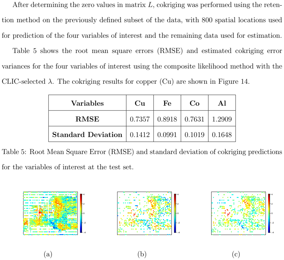
Estimating covariance parameters for multivariate spatial Gaussian random fields is computationally challenging, as the number of parameters grows rapidly with the number of variables, and likelihood evaluation requires operations of order $\mathcal{O}((np)^3)$. In many applications, however, not all cross-dependencies between variables are relevant, suggesting that sparse covariance structures may be both statistically advantageous and practically necessary. We propose a LASSO-penalized estimation framework that induces sparsity in the Cholesky factor of the multivariate Mat\'{e}rn correlation matrix, enabling automatic identification of uncorrelated variable pairs while preserving positive semidefiniteness. Estimation is carried out via a projected block coordinate descent algorithm that decomposes the optimization into tractable subproblems, with constraints enforced at each iteration through appropriate projections. Regularization parameter selection is discussed for both the likelihood and composite likelihood approaches. We conduct a simulation study demonstrating the ability of the method to recover sparse correlation structures and reduce estimation error relative to unpenalized approaches. We illustrate our procedure through an application to a geochemical dataset with $p = 36$ variables and $n = 3998$ spatial locations, showing the practical impact of the method and making spatial prediction feasible in a setting where standard approaches fail entirely.
Editorial analysis
A structured set of objections, weighed in public.
Referee Report
Summary. The manuscript proposes a LASSO-penalized likelihood framework for estimating covariance parameters in highly multivariate spatial Gaussian random fields under the multivariate Matérn model. Sparsity is induced in the Cholesky factor L of the p × p correlation matrix R = L L^T via penalized estimation, with positive semidefiniteness preserved by a projected block coordinate descent algorithm. The approach is claimed to enable automatic identification of uncorrelated variable pairs. Regularization parameter selection is discussed for both full and composite likelihoods. A simulation study is presented to show recovery of sparse structures and reduced estimation error, together with a real-data application to a geochemical dataset (p = 36 variables, n = 3998 locations) where unpenalized methods are infeasible.
Significance. If the central mapping from sparsity in L to interpretable uncorrelated pairs holds without distorting the Matérn parameters or spatial dependence, the method would address a genuine computational barrier in high-dimensional spatial statistics and make likelihood inference practical for large p. The projected block coordinate descent and composite-likelihood option are pragmatic strengths. However, the interpretation gap between L-sparsity and R-sparsity (zero cross-covariances) limits the strength of the claims until addressed.
major comments (1)
- [Abstract] Abstract: the central claim that the LASSO penalty on the Cholesky factor 'enables automatic identification of uncorrelated variable pairs' does not follow from the construction. Because R = L L^T, zeroing selected entries of L does not force the corresponding entries of R to zero; nonzero cross terms can remain. The simulation claim of 'recovering sparse correlation structures' therefore rests on an unverified assumption that L-sparsity produces the intended R-sparsity. This is load-bearing for the paper's interpretation and must be corrected or demonstrated explicitly (e.g., by reporting the sparsity pattern of the estimated R and verifying that cross-covariance functions are effectively zero).
minor comments (1)
- The abstract states that regularization parameter selection is discussed for both likelihood and composite likelihood, but the concrete criteria (e.g., BIC, cross-validation, or information criteria) and their finite-sample behavior should be stated more explicitly.
Simulated Author's Rebuttal
We thank the referee for the careful and constructive review of our manuscript. The major comment highlights an important distinction between sparsity in the Cholesky factor L and exact sparsity in the correlation matrix R. We address this point directly below and commit to revisions that clarify the claims and provide explicit verification.
read point-by-point responses
-
Referee: [Abstract] Abstract: the central claim that the LASSO penalty on the Cholesky factor 'enables automatic identification of uncorrelated variable pairs' does not follow from the construction. Because R = L L^T, zeroing selected entries of L does not force the corresponding entries of R to zero; nonzero cross terms can remain. The simulation claim of 'recovering sparse correlation structures' therefore rests on an unverified assumption that L-sparsity produces the intended R-sparsity. This is load-bearing for the paper's interpretation and must be corrected or demonstrated explicitly (e.g., by reporting the sparsity pattern of the estimated R and verifying that cross-covariance functions are effectively zero).
Authors: We agree that exact zeros in L do not mathematically guarantee exact zeros in R, since the (i,j) entry of R is the dot product of the i-th and j-th rows of L. Our approach uses the Cholesky parameterization primarily to enforce positive definiteness during penalized estimation, while the LASSO penalty on L encourages many zero entries that, in practice, drive the corresponding cross terms in R to be very small. This enables effective identification of pairs with negligible cross-dependence for the purposes of high-dimensional spatial modeling. Nevertheless, we acknowledge that the original wording in the abstract overstated the direct implication. In the revised manuscript we will (i) rephrase the abstract to state that the penalized Cholesky approach induces sparsity in L and thereby facilitates recovery of approximately sparse correlation structures, and (ii) add explicit verification in the simulation section by reporting the sparsity patterns (number of exact or near-zero entries) of both the estimated L and R matrices, together with numerical checks that the cross-covariance functions for the identified pairs fall below a small threshold (e.g., 0.01). These additions will directly address the referee's suggestion and strengthen the interpretability of the results. revision: yes
Circularity Check
No significant circularity; method is a standard penalized likelihood with independent parameterization
full rationale
The paper introduces a LASSO penalty on the Cholesky factor of the multivariate Matérn correlation matrix and uses projected block coordinate descent for estimation. No step reduces by construction to a fitted parameter renamed as a prediction, nor does any central claim rely on a self-citation chain that is itself unverified or load-bearing. The claim that sparsity in the Cholesky factor enables identification of uncorrelated pairs is a methodological assertion about the procedure's effect rather than an equivalence derived from the paper's own equations. The simulation and application sections provide empirical support outside the fitting process itself. The derivation remains self-contained against external benchmarks.
Axiom & Free-Parameter Ledger
free parameters (1)
- LASSO regularization parameter
axioms (2)
- standard math Multivariate Matérn correlation functions produce positive semidefinite matrices
- domain assumption Sparsity in the Cholesky factor identifies uncorrelated variable pairs
Reference graph
Works this paper leans on
-
[1]
By conditions (C2) and (C3), the mappingθ7→Q(h;θ) is continuous with continuous derivative. SinceU N(θ) andK(θ, θ 0) (defined in Equation (17)) are compositions of continuous functions, they are themselves continuous
-
[2]
The weak law of large numbers together with condition C1 implies that, asN→ ∞, bQ(h)→Q(h;θ 0) in probability. Therefore, ˜UN converges in probability toK(θ, θ 0) (defined in (17)), which has a unique minimum atθ 0 by condition C4. 43
-
[3]
1 2 n−1X k=1 nX l=k+1 tr Q−1 kl ∂Qkl ∂θh1 Q−1 kl ∂Qkl ∂θh2 #q h1,h2=1 (29) J(θ) =
Define the modulus of continuity of ˜UN(θ) as WN(η) = sup ∥α−β∥≤η ˜UN(α)− ˜UN(β) , α, β∈Θ.(18) Then we have ˜UN(α)− ˜UN(β) ≤ X h∈M log |Q(h;α)| |Q(h;β)| + tr bQ(h) Q−1(h;α)−Q −1(h;β) .(19) By conditions (C2) and (C3), the functionsθ7→Q(h;θ) are Lipschitz; then, by composition of Lipschitz functions, we have X h∈M log |Q(h;α)| |Q(h;β)| ≤ " L1 + X h∈M L2 # ...
work page 2016
discussion (0)
Sign in with ORCID, Apple, or X to comment. Anyone can read and Pith papers without signing in.