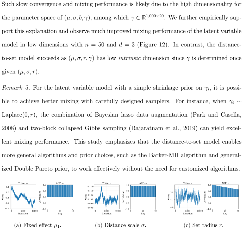
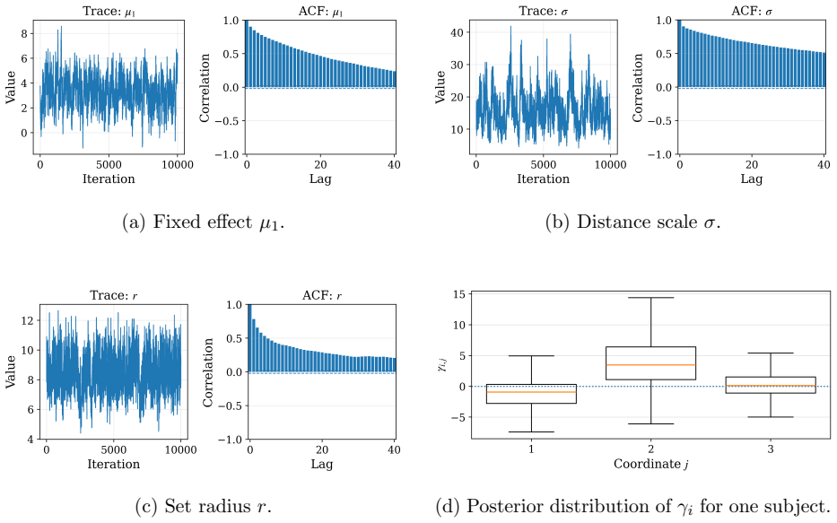
Bayesian Distance-to-Set Models: from Latent Variable to Latent Projection
Pith reviewed 2026-05-10 15:46 UTC · model grok-4.3
The pith
Bayesian models replace latent coordinates with projections onto sets to shrink the latent space and speed up sampling.
A machine-rendered reading of the paper's core claim, the machinery that carries it, and where it could break.
Core claim
The paper claims that distance-to-set models, in which the likelihood is written in terms of the distance from each observation to its projection onto the target set rather than deviation from a latent coordinate, reduce the dimensionality of the latent-variable space, permit efficient posterior computation via optimization-based projections, and satisfy the statistical properties of independence between normal-cone noise and fixed-effect parameters, posterior consistency, and an Occam's-razor effect that penalizes overfitting.
What carries the argument
The distance-to-set, defined as the distance between a data point and its projection onto the structured set, with the projection computed by optimization and inserted in place of the latent coordinate.
If this is right
- Posterior sampling remains feasible for large sample sizes even when no closed-form marginalization of latent variables exists.
- Normal-cone noise is independent of fixed-effect parameters.
- Posterior consistency is preserved.
- The model automatically penalizes overfitting.
Where Pith is reading between the lines
- The approach may extend naturally to other structured-data problems where projections onto the same sets are already computable.
- It could be combined with existing fast optimization routines to handle higher-dimensional or non-Euclidean sets.
- Similar dimensionality reduction might be tested in frequentist estimation settings that also rely on proximity to low-dimensional sets.
Load-bearing premise
The projection of each data point onto the set of interest can be computed rapidly and accurately by optimization for the sets that arise in practice.
What would settle it
Apply the distance-to-set sampler to a large dataset whose set projections require many iterations or fail to converge reliably, then compare the mixing time and coverage of credible intervals against a standard latent-variable MCMC run on the same data.
Figures


read the original abstract
Statistical models often assume that data are generated near a structured, smooth, or low-dimensional set. A common approach is to use Bayesian latent variable models, in which each observation is associated with a latent coordinate on the set, and the observed data are modeled as noisy deviations from these coordinates. The deviation is typically characterized by a location-scale distribution, such as Gaussian. Despite their intuitive appeal and popularity, latent variable models often present practical challenges in posterior computation. In particular, Markov chain Monte Carlo samplers may suffer from slow mixing, especially when the sample size is large and there is no closed form for integrating out the latent coordinates. In this article, we propose an alternative approach that replaces the deviation-from-coordinate with a distance-to-set. Specifically, the distance-to-set is defined as the distance between a data point and its projection onto the set, where the projection can be rapidly computed by optimization and replaces the latent coordinate in the likelihood. This change substantially reduces the dimensionality of the parameter X latent variable space, leading to efficient posterior computation. We establish several important statistical properties for the distance-to-set models, such as the independence between the normal-cone noise and fixed-effect parameters, posterior consistency, and an Occam's razor effect that automatically penalizes overfitting. We demonstrate the effectiveness of our approach through simulation studies, applications to multi-environment study and Bayesian transfer learning.
Editorial analysis
A structured set of objections, weighed in public.
Referee Report
Summary. The manuscript proposes Bayesian distance-to-set models as an alternative to traditional latent variable models for data generated near structured sets. Rather than modeling observations as noisy deviations from latent coordinates on the set, the approach replaces the latent coordinate with the distance to the data point's projection onto the set, where the projection is obtained via optimization. This substitution reduces the dimensionality of the latent space, enabling more efficient posterior computation. The authors establish statistical properties including independence of normal-cone noise from fixed-effect parameters, posterior consistency, and an automatic Occam's razor penalty for overfitting. Effectiveness is demonstrated via simulation studies and applications to multi-environment studies and Bayesian transfer learning.
Significance. If the claimed properties hold and projections remain computationally tractable, the framework offers a scalable alternative for Bayesian modeling of structured data, addressing slow mixing in high-dimensional latent variable settings while retaining key inferential guarantees. The explicit dimensionality reduction and derived theoretical results (consistency, noise independence, automatic regularization) constitute a substantive contribution to computational statistics.
minor comments (4)
- Clarify the precise definition of the distance-to-set and its relation to the normal cone in the likelihood construction; the abstract introduces these terms without an explicit equation, which may confuse readers unfamiliar with set-valued projections.
- In the simulation studies, report wall-clock times or effective sample sizes alongside the efficiency claims to quantify the posterior computation gains relative to standard latent variable MCMC.
- The Occam's razor effect is asserted to automatically penalize overfitting; provide a brief comparison (e.g., via marginal likelihood or posterior predictive checks) against a baseline latent variable model to illustrate this property empirically.
- Ensure all applications (multi-environment study, transfer learning) include sufficient detail on the specific sets used and how projections are computed, including any convergence diagnostics for the optimization step.
Simulated Author's Rebuttal
We thank the referee for their positive assessment of the manuscript, accurate summary of the proposed Bayesian distance-to-set framework, and recommendation for minor revision. The significance statement correctly identifies the dimensionality reduction, computational benefits, and theoretical guarantees (posterior consistency, noise independence, and automatic regularization) as the core contributions.
Circularity Check
No significant circularity in derivation chain
full rationale
The paper proposes a modeling shift from latent-variable coordinates on a set to distance-to-set via deterministic projections computed by optimization. This reduces the latent space dimension and yields a likelihood depending on scalar distances plus normal-cone residuals. The abstract and description present posterior consistency, normal-cone independence from fixed effects, and an automatic Occam penalty as consequences of the new formulation rather than inputs. No equations are shown that reduce by construction to fitted parameters, no self-definitional loops, and no load-bearing self-citations or ansatzes imported from prior author work. The derivation remains self-contained against external benchmarks at the level of the given text.
Axiom & Free-Parameter Ledger
free parameters (1)
- scale parameter in distance distribution
axioms (2)
- domain assumption The structured set admits a well-defined projection that can be rapidly computed via optimization
- domain assumption The deviation can be modeled as normal-cone noise independent of fixed effects
Reference graph
Works this paper leans on
-
[1]
PMLR. Xu, J., E. C. Chi, M. Yang, and K. Lange (2018). A majorization–minimization algorithm for split feasibility problems.Computational Optimization and Applications 71(3), 795– 828. Zens, G., S. Fr¨ uhwirth-Schnatter, and H. Wagner (2024). Ultimate P´ olya Gamma Samplers–Efficient MCMC for Possibly Imbalanced Binary and Categorical Data.Jour- nal of th...
work page 2018
-
[2]
(23) Thus, reconstruction-based learning procedures can be interpreted as giving rise to divergence- to-set models or vice versa, in which the reconstruction map plays the role of a tractable 47 surrogate projection. This perspective suggests that a range of popular machine learning procedures may be embedded into the divergence-to-set framework. 8.6 Samp...
work page 2013
-
[3]
and two-block collapsed Gibbs sampling (Rajaratnam et al., 2019) can yield excel- lent mixing performance. This study emphasizes that the distance-to-set model enables more general algorithms and prior choices, such as the Barker-MH algorithm and general- ized Double Pareto prior, to work effectively without the need for customized algorithms. (a) Fixed e...
work page 2019
discussion (0)
Sign in with ORCID, Apple, or X to comment. Anyone can read and Pith papers without signing in.