arxiv: 2604.14043 · v1 · submitted 2026-04-15 · 🌌 astro-ph.SR

Recognition: unknown

Non-LTE Analysis of Pre-eruptive Prominence Plasma Parameters Effects on the Lyman-beta and Lyman-gamma Lines with Solar Orbiter SPICE Observations

Yong Zhang (1) , Nicolas Labrosse (1) , Susanna Parenti (2 , 3) , Therese A. Kucera (4) ((1) SUPA School of Physics , Astronomy , University of Glasgow , Glasgow G12 8QQ UK

show 16 more authors

(2) Institut d'Astrophysique Spatiale Bat 121 Universit\'e Paris-Saclay/CNRS 91405 Orsay Cedex France (3) Universit\'e Paris-Saclay Universit\'e Paris Cit\'e CEA CNRS AIM 91191 Gif-sur-Yvette France (4) Heliophysics Science Division NASA Goddard Space Flight Center Greenbelt MD 20771 USA)

Authors on Pith no claims yet

Pith reviewed 2026-05-10 11:50 UTC · model grok-4.3

classification 🌌 astro-ph.SR

keywords prominenceLyman linesnon-LTESolar OrbiterSPICEplasma parametersline formation

0 comments

The pith

Non-LTE models constrained by Solar Orbiter observations identify central pressure, column mass, and temperature gradient as the main controls on Lyman-beta and Lyman-gamma line formation in prominences.

A machine-rendered reading of the paper's core claim, the machinery that carries it, and where it could break.

The paper examines the first dedicated off-limb prominence observation by Solar Orbiter on April 15, 2023. It creates 200 random non-LTE models that respect the available SPICE spectral constraints and an incident-radiation field taken from a full-disk mosaic. Lyman beta and gamma line profiles are computed for each model, and parallel coordinate plots display how the input parameters map onto the output profiles. This procedure isolates the physical quantities that most strongly shape the observed lines. Readers interested in solar plasma diagnostics would see a concrete route from spectral data to refined estimates of prominence conditions.

Core claim

The paper shows that an ensemble of 200 random non-LTE models, bounded by SPICE observations of a pre-eruptive prominence and by incident radiation derived from a November 13, 2023 full-disk mosaic, yields clear inferences about the central pressure, column mass, and temperature gradient that govern the formation of the Lyman beta and Lyman gamma lines.

What carries the argument

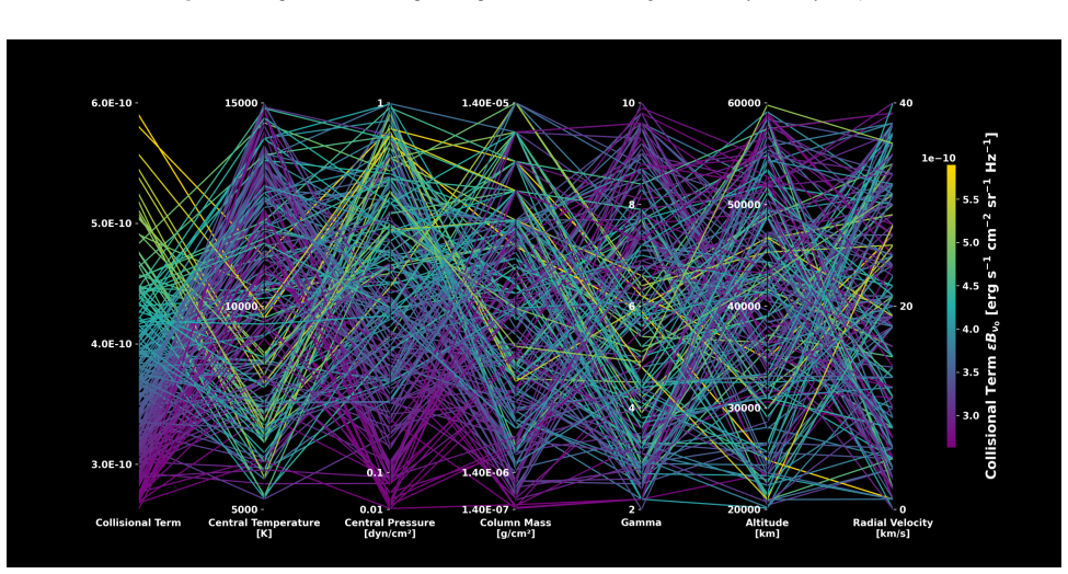
The 200 randomly sampled non-LTE models, each constrained by the SPICE spectral data and the chosen incident-radiation mosaic, used to generate Lyman beta and gamma profiles and to map parameter influence via parallel coordinate plots.

Load-bearing premise

The 200 randomly generated models, limited only by the SPICE observations and one incident-radiation mosaic, are assumed to sample the full range of physically realistic conditions.

What would settle it

A direct comparison between the observed SPICE Lyman-beta and Lyman-gamma profiles and the synthetic profiles produced by the subset of models whose central pressure, column mass, and temperature gradient fall inside the inferred ranges.

Figures

Figures reproduced from arXiv: 2604.14043 by 20771 USA), (2) Institut d'Astrophysique Spatiale, 3), (3) Universit\'e Paris-Saclay, (4) Heliophysics Science Division, 91191, AIM, Astronomy, Bat 121, CEA, CNRS, France, Gif-sur-Yvette, Glasgow G12 8QQ UK, Greenbelt, MD, NASA Goddard Space Flight Center, Nicolas Labrosse (1), Susanna Parenti (2, Therese A. Kucera (4) ((1) SUPA School of Physics, Universit\'e Paris Cit\'e, Universit\'e Paris-Saclay/CNRS 91405 Orsay Cedex France, University of Glasgow, Yong Zhang (1).

**Figure 1.** Figure 1: The SPICE observation of the integrated intensity of the Lyman 𝛽 and Lyman 𝛾 lines taken from 07:03:40 - 08:09:23 UT, 15 April 2023. The red rectangle is the prominence region we study. and 𝑛 = 4 energy levels to the ground state (𝑛 = 1), respectively. They are strong lines and well suited to study chromospheric plasmas, especially prominences (Heinzel et al. 2001). 2.2 Observations The prominence, a large… view at source ↗

**Figure 2.** Figure 2: The solar map of the integrated intensity of the H-Lyman 𝛽 line by SPICE full disc mosaic observation on Nov 13∼14, 2023. from the eruption. In [PITH_FULL_IMAGE:figures/full_fig_p003_2.png] view at source ↗

**Figure 3.** Figure 3: The red points are the incident Lyman 𝛽 line profile we obtained following the method of Zhang (2019) with SPICE full disc mosaic observation on Nov 13–14, 2023, and the orange line is the Gaussian fit of the red points. The green line is the average line profile within the 50 arcsec of the solar center in the mosaic image. The blue line is the incident Lyman 𝛽 line profile in the PRODOP NLTE code. It is … view at source ↗

**Figure 4.** Figure 4: The parallel coordinate plot of 4 parameters with the integrated intensity of the H𝛼 line. In a parallel coordinate plot, if we see a diversity of colours connected to different value ranges when we focus on one parameter’s axis, this means the parameter does not have much effect; on the other hand, if we see a certain colour concentrated on a certain value range, this means the parameter has some effect. … view at source ↗

**Figure 5.** Figure 5: Integrated intensity vs. emission measure, temperature, pressure and slab thickness for the H𝛼 line. We divided the range of each x-axis parameter (log EM, log T, log p, log ST) into 50 bins. For each bin, all models falling inside it (the number varies across bins) were averaged in log E(H𝛼), and only bins containing data are shown. • We can understand the sensitivity of the property that determines the … view at source ↗

**Figure 6.** Figure 6: The parallel coordinate plot of 6 parameters with the integrated intensity of the Lyman 𝛽 line [PITH_FULL_IMAGE:figures/full_fig_p006_6.png] view at source ↗

**Figure 7.** Figure 7: The parallel coordinate plot of 6 parameters with the collisional term 𝜖 𝐵𝜈0 of the Lyman 𝛽 line. the change of this parameter, which means that it has a high elasticity coefficient. 4 RESULTS 4.1 Effects of model parameters on Lyman line properties Using the altitude and incident radiation constraints as described in Section 2.2 and Section 3.1, the radial velocity constraint from Zhang et al. (2026), and… view at source ↗

**Figure 8.** Figure 8: The parallel coordinate plot of 6 parameters with the radiation term (1 − 𝜖 ) 𝐽¯ of the Lyman 𝛽 line [PITH_FULL_IMAGE:figures/full_fig_p007_8.png] view at source ↗

**Figure 9.** Figure 9: The parallel coordinate plot of 6 parameters with the optical thickness of the Lyman 𝛽 line. coefficients smaller than 0.3 and their elasticity coefficients are generally smaller than the lowest values listed in the tables. However, there are exceptions. For example, the elasticity coefficient of central temperature for the radiation term in Lyman 𝛽 and Lyman 𝛾 lines is very closed to that of column mass … view at source ↗

**Figure 10.** Figure 10: The parallel coordinate plot of 6 parameters with the integrated intensity of the Lyman 𝛾 line [PITH_FULL_IMAGE:figures/full_fig_p008_10.png] view at source ↗

**Figure 11.** Figure 11: The parallel coordinate plot of 6 parameters with the collisional term 𝜖 𝐵𝜈0 of the Lyman 𝛾 line. For the radiation term (1 − 𝜖)𝐽¯, higher central pressure or larger column mass is also generally associated with a larger radiation term, whereas larger 𝛾 values lead to smaller values of the radiation term. For the optical thickness, an increase in central temperature tends to reduce optical thickness in bo… view at source ↗

**Figure 12.** Figure 12: The parallel coordinate plot of 6 parameters with the radiation term (1 − 𝜖 ) 𝐽¯ of the Lyman 𝛾 line [PITH_FULL_IMAGE:figures/full_fig_p009_12.png] view at source ↗

**Figure 13.** Figure 13: The parallel coordinate plot of 6 parameters with the optical thickness of the Lyman 𝛾 line. mass and gamma. In [PITH_FULL_IMAGE:figures/full_fig_p009_13.png] view at source ↗

**Figure 14.** Figure 14: The probability distribution of the central pressure refined by observation [PITH_FULL_IMAGE:figures/full_fig_p010_14.png] view at source ↗

**Figure 15.** Figure 15: The probability distribution of the central temperature refined by observation. term 𝜖 𝐵𝜈0 and radiation term (1 − 𝜖)𝐽¯ have a similar distribution of values. This suggests that collisional contribution and radiative contribution are equally important for the formation of the Lyman 𝛾 line. In Figures 13, we can see that all yellow lines (optical thickness larger than 1000) distribute below 10000 K on the … view at source ↗

**Figure 16.** Figure 16: The probability distribution of the Lyman 𝛽 line optical thickness refined by observation [PITH_FULL_IMAGE:figures/full_fig_p011_16.png] view at source ↗

**Figure 17.** Figure 17: The probability distribution of the Lyman 𝛾 line optical thickness refined by observation. the requirement. We find that 36 of them have a central pressure below 0.48 dyn cm−2 . However, we find that the column mass and gamma of these models seem to have a nearly equal possibility of being distributed in each value within the range after restricting the integrated intensity of the Lyman 𝛽 and Lyman 𝛾 line… view at source ↗

read the original abstract

The first dedicated observation of an off-limb prominence by Solar Orbiter took place on April 15, 2023. Our aim is to determine the range of different physical parameters of this prominence and to examine how these parameters affect the formation of the Lyman $\beta$ and Lyman $\gamma$ lines of hydrogen. We have found a way to refine key physical parameters by observational data. We will test the method by this prominence observation. We generate 200 random non-LTE models using these observational constraints and compute the Lyman $\beta$ line and the Lyman $\gamma$ line profiles. We use the Spectral Imaging of the Coronal Environment (SPICE) full-disk mosaic from November 13, 2023 to constrain the incident radiation. We present the parameters and results of 200 random models using parallel coordinate plots to explore how different parameters affect the results. This allows us to infer the key physical parameters (e.g., central pressure, column mass and temperature gradient) that impact the formation of the Lyman $\beta$ line and the Lyman $\gamma$ line in this observation.

Editorial analysis

A structured set of objections, weighed in public.

Desk editor's note, referee report, simulated authors' rebuttal, and a circularity audit. Tearing a paper down is the easy half of reading it; the pith above is the substance, this is the friction.

Desk Editor's Note private letter to a colleague

The paper applies non-LTE modeling to the first dedicated SPICE off-limb prominence observation but 200 random models leave the parameter space too thinly sampled to support firm claims about which parameters control the Lyman lines.

read the letter

The main takeaway is that this work takes the April 15 2023 off-limb prominence data from Solar Orbiter SPICE and runs 200 random non-LTE models constrained by those observations plus a November incident-radiation mosaic, then uses parallel-coordinate plots to explore effects on the Lyman beta and gamma profiles. The authors conclude that central pressure, column mass, and temperature gradient are the key parameters to infer from this kind of data. That is the practical step they are offering for future SPICE prominence work. What is actually new here is the application to this specific first dedicated off-limb SPICE dataset rather than any new modeling technique or theoretical result. The existing non-LTE prominence codes are used in a standard way, and the parallel plots are a common visualization tool, but tying them to real SPICE Lyman-line observations is a fresh data point for the community. The paper does a clear job of stating the observational constraints and showing the spread of model outputs, which at least gives readers a concrete sense of how the lines respond across the sampled range. The soft spots are mainly around coverage and validation. Three hundred models would still be modest in a space with central pressure, column mass, temperature gradient, and any additional free parameters, so large regions remain unexplored and any apparent key parameters could shift with denser sampling. The abstract gives no quantitative fit metrics, no residuals, and no recovery tests on synthetic data with known inputs, which makes it hard to judge how well the models actually reproduce the observed profiles or how unique the inferred values are. The incident radiation is taken from a different date, adding an untested assumption about stability. This paper is aimed at solar-atmosphere modelers who work on prominences and Lyman-line diagnostics, especially those planning or analyzing SPICE observations. A reader who wants a practical example of ensemble exploration on new data will find something useful in the figures and setup. It is solid enough on the data side and honest in its engagement with the literature to deserve a serious referee, though the review will probably focus on sampling density and the need for fit statistics. I would send it out for peer review with requests for those additions rather than desk-rejecting it.

Referee Report

4 major / 2 minor

Summary. The paper analyzes the first off-limb prominence observation by Solar Orbiter SPICE on 15 April 2023. It generates 200 random non-LTE models constrained by the SPICE data and a November 13 incident-radiation mosaic, computes the resulting Lyman β and Lyman γ line profiles, and employs parallel-coordinate plots to identify which parameters (central pressure, column mass, temperature gradient) most strongly affect the line formation.

Significance. If the sampling and inference procedure were shown to be robust, the work would demonstrate a practical route to constraining prominence plasma parameters from Lyman-line observations with SPICE, adding a new diagnostic tool for solar-atmosphere studies. The approach is novel in its use of an ensemble of random models tied directly to a specific SPICE dataset.

major comments (4)

[Abstract] Abstract and method description: the central claim that 200 randomly generated models suffice to 'infer the key physical parameters' is not supported by any quantitative goodness-of-fit metric (e.g., χ², residual maps, or intensity ratios) between the computed and observed line profiles, nor by error bars or posterior distributions on the inferred parameters.
[Abstract] Abstract: the Monte-Carlo sampling of the three-dimensional parameter space (central pressure, column mass, temperature gradient) with only 200 draws is too sparse to guarantee that the regions reproducing the observed Lyman β/γ profiles are uniquely identified; no convergence test or comparison with a larger ensemble is presented.
[Abstract] Abstract: the incident radiation is taken from a full-disk mosaic acquired on 13 November 2023, seven months after the 15 April prominence observation; no assessment of temporal variability or its effect on the derived line profiles is provided, undermining the reliability of the model-observation comparison.
[Abstract] Abstract: no forward-modeling test with synthetic observations of known input parameters is reported, leaving open the possibility that the parallel-coordinate analysis recovers spurious 'key' parameters due to the limited sampling and the circular use of the same data for both constraint and inference.

minor comments (2)

[Abstract] The abstract states that the models are 'constrained by these observational constraints' without specifying the exact observational quantities (e.g., which SPICE spectral windows or spatial pixels) used to set the random-model bounds.
[Abstract] Parallel-coordinate plots are mentioned but no figure numbers, axis ranges, or selection criteria for 'key' parameters are given in the provided text.

Simulated Author's Rebuttal

4 responses · 0 unresolved

We thank the referee for the constructive and detailed report. We address each major comment below, indicating where revisions will be made to improve the manuscript's rigor and clarity.

read point-by-point responses

Referee: [Abstract] Abstract and method description: the central claim that 200 randomly generated models suffice to 'infer the key physical parameters' is not supported by any quantitative goodness-of-fit metric (e.g., χ², residual maps, or intensity ratios) between the computed and observed line profiles, nor by error bars or posterior distributions on the inferred parameters.

Authors: We agree that the current analysis relies primarily on parallel-coordinate plots for identifying influential parameters rather than formal statistical fitting. The 200 models were generated subject to the SPICE observational constraints, but quantitative metrics were not computed. In the revised manuscript we will add χ² values, residual maps, and intensity-ratio comparisons for the subset of models that best reproduce the observed Lyman-β and Lyman-γ profiles, together with simple uncertainty estimates derived from the ensemble spread. revision: yes
Referee: [Abstract] Abstract: the Monte-Carlo sampling of the three-dimensional parameter space (central pressure, column mass, temperature gradient) with only 200 draws is too sparse to guarantee that the regions reproducing the observed Lyman β/γ profiles are uniquely identified; no convergence test or comparison with a larger ensemble is presented.

Authors: We acknowledge that 200 samples provide only an exploratory view of the three-dimensional parameter space. To demonstrate robustness we will repeat the analysis with a larger ensemble (1000 models) and include a convergence test showing that the ranking of key parameters (central pressure, column mass, temperature gradient) remains stable. This comparison will be added to the methods and results sections. revision: yes
Referee: [Abstract] Abstract: the incident radiation is taken from a full-disk mosaic acquired on 13 November 2023, seven months after the 15 April prominence observation; no assessment of temporal variability or its effect on the derived line profiles is provided, undermining the reliability of the model-observation comparison.

Authors: The November 2023 mosaic was the nearest available full-disk dataset suitable for constraining the incident radiation field. We will expand the discussion to note the seven-month separation and to reference typical timescales of solar EUV variability. A quantitative assessment of variability effects would require contemporaneous full-disk observations that are not available for this event; we will therefore treat this as an explicit limitation of the present study. revision: partial
Referee: [Abstract] Abstract: no forward-modeling test with synthetic observations of known input parameters is reported, leaving open the possibility that the parallel-coordinate analysis recovers spurious 'key' parameters due to the limited sampling and the circular use of the same data for both constraint and inference.

Authors: We recognize the value of an independent validation step. In the revised manuscript we will add a forward-modeling test: synthetic Lyman-β and Lyman-γ profiles will be generated from a known set of input parameters, then recovered using the same 200-model ensemble and parallel-coordinate procedure. This will demonstrate that the method correctly identifies the injected key parameters and will be presented as a new subsection. revision: yes

Circularity Check

0 steps flagged

No circularity: forward modeling within observational constraints

full rationale

The paper generates 200 random non-LTE models constrained by SPICE off-limb observations from April 15 2023 and a separate November 13 mosaic for incident radiation, then computes synthetic Lyman β and γ profiles and uses parallel-coordinate plots to examine how parameters such as central pressure, column mass and temperature gradient affect those computed profiles. This is a standard forward-modeling parameter-space exploration; the line profiles are outputs of the radiative-transfer calculation, not inputs that are fitted and then re-labeled as predictions. No self-citations, self-definitional steps, uniqueness theorems, or renamings of known results appear in the provided text, so the derivation chain remains self-contained.

Axiom & Free-Parameter Ledger

3 free parameters · 2 axioms · 0 invented entities

The work rests on standard non-LTE radiative-transfer assumptions and the representativeness of the chosen incident-radiation mosaic. No new particles or forces are introduced. Free parameters are the randomly sampled physical quantities whose ranges are set by observational constraints.

free parameters (3)

central pressure
Sampled randomly within observational bounds; directly affects line formation.
column mass
Sampled randomly; controls optical depth and line strength.
temperature gradient
Sampled randomly; shapes the height-dependent excitation.

axioms (2)

domain assumption Non-LTE conditions govern the formation of Lyman-beta and Lyman-gamma lines in the prominence plasma.
Invoked throughout the modeling section; standard in solar-atmosphere work but not re-derived here.
domain assumption The November 13 2023 SPICE full-disk mosaic provides a representative incident radiation field for the April 15 prominence.
Used to constrain the models; temporal mismatch is not quantified.

pith-pipeline@v0.9.0 · 5642 in / 1644 out tokens · 23496 ms · 2026-05-10T11:50:44.819187+00:00 · methodology

discussion (0)

Reference graph

Works this paper leans on

1 extracted references · 1 canonical work pages

[1]

Anderson M., et al., 2020, A&A, 642, A14 Anzer U., Heinzel P., 1999, A&A, 349, 974 DufresneR.,DelZannaG.,YoungP.,DereK.,DeliporanidouE.,BarnesW., Landi E., 2024, The Astrophysical Journal, 974, 71 Edsall R. M., 2003, Computational Statistics & Data Analysis, 43, 605 GeY.,LiS.,LakhanV.C.,LucieerA.,2009,InternationalJournalofApplied Earth Observation and Ge...

work page doi:10.1007/978-3-319-10416-4 2020