A critical note on back-and-forth Data Assimilation Nudging Algorithm
Pith reviewed 2026-05-10 01:20 UTC · model grok-4.3
The pith
Back-and-forth nudging cannot reliably recover initial conditions from sparse observations in dissipative systems.
A machine-rendered reading of the paper's core claim, the machinery that carries it, and where it could break.
Core claim
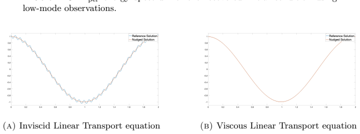
For several dissipative systems, infinitely many distinct solutions share identical spatially sparse observational data. The BFN algorithm, which relies on nudging based on these observations, therefore cannot recover the true initial condition or differentiate between these solutions. This is demonstrated analytically for the Lorenz 1963 model, the heat equation, viscous linear transport, and viscous and inviscid Burgers equations, with supporting numerical simulations. A Voigt-regularized BFN is introduced to address ill-posedness in backward iterations for the 2D Navier-Stokes equations and viscous KdV equation, yet it remains limited in reconstructing the full state from sparse data.
What carries the argument
The explicit construction of infinitely many distinct solutions that produce identical spatially sparse observational data, which prevents any observation-dependent nudging scheme from enforcing uniqueness of the initial condition.
Load-bearing premise
Spatially sparse observational data is sufficient to uniquely determine the solution trajectory among different possible initial conditions in the dissipative systems considered.
What would settle it
Numerical simulation of the Lorenz model or Burgers equation showing whether two different initial conditions that are constructed to match at the sparse observation locations remain indistinguishable in their observed values while diverging in unobserved regions.
Figures


read the original abstract
This work investigates the effectiveness of the Back-and-Forth Nudging (BFN) data assimilation algorithm, specifically its performance when employing the Azouani-Olson-Titi (AOT) continuous data assimilation downscaling nudging algorithm, for recovering initial conditions of dissipative dynamical systems. Contrary to previous reports in the literature, we show that, for several systems of interest, one can construct initial conditions that BFN cannot reliably recover. Our key finding is the construction of infinitely many distinct solutions for certain dissipative systems that share identical spatially sparse observational data. Since these observations are indistinguishable, no data assimilation method relying only on them can differentiate between these solutions or recover the correct initial condition. We illustrate these pathological initial conditions for the Lorenz 1963 model and several 1D partial differential equations: the heat equation, viscous linear transport, and viscous and inviscid Burgers equations. Our analytical results are supported by numerical simulations. To address the numerical ill-posedness of backward-in-time iterations, an essential step of BFN for dissipative models, we introduce a regularized backward step, the Voigt-regularized BFN (VBFN). We investigate its performance for the 2D Navier-Stokes equations and the viscous 1D KdV equation, comparing it with standard BFN and Diffusive BFN (dBFN). While VBFN improves numerical stability and reduces model bias relative to dBFN, it still cannot reconstruct the unobserved fine spatial scales of the reference solution. This reinforces our main conclusion: even with regularization, BFN-type algorithms are limited in recovering the full state, and in particular the initial data, from sparse spatial observations.
Editorial analysis
A structured set of objections, weighed in public.
Referee Report
Summary. The paper claims that Back-and-Forth Nudging (BFN) and its variants cannot reliably recover initial conditions for dissipative systems (Lorenz 1963, heat, viscous transport, viscous/inviscid Burgers) under spatially sparse continuous-in-time observations, because one can construct infinitely many distinct solutions sharing identical data; the nudging term vanishes on this family since it depends only on pointwise differences at observed locations. Analytical constructions are asserted for each system and supported by numerical simulations. To mitigate backward-step ill-posedness, the authors introduce Voigt-regularized BFN (VBFN) and compare it with standard BFN and diffusive BFN on 2D Navier-Stokes and 1D viscous KdV, concluding that regularization improves stability but does not recover unobserved fine scales.
Significance. If the non-uniqueness constructions are made fully explicit, the work identifies a concrete limitation of nudging-based DA: the observation operator has a non-trivial kernel for standard sparse point measurements, so any method using only those data cannot select a unique initial condition. The direct kernel argument (superposition of null-space components) is a strength, as is the introduction of VBFN for numerical stability. This could prompt re-examination of observation density requirements in DA literature and encourage hybrid schemes that add constraints beyond pointwise nudging.
major comments (3)
- [Analytical constructions (heat equation)] § on heat-equation construction: the assertion that higher eigenmodes (odd with respect to interior observation points) lie in the kernel and can be superposed while preserving observations is central, yet no explicit non-trivial example is supplied (e.g., a concrete eigenfunction, observation point x0, and verification that the solution satisfies the PDE and matches data for all t). Without this, the claim that the nudging term vanishes identically remains difficult to verify.
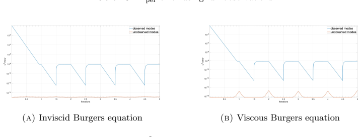
- [Numerical results] Numerical simulations section: the manuscript states that simulations support the analytical non-uniqueness, but provides neither the precise definition of the discrete observation operator, the time-stepping scheme, nor quantitative error metrics (L2 or pointwise differences between recovered and reference trajectories) in the figures or tables. This weakens the evidential link between analysis and numerics.
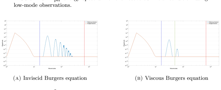
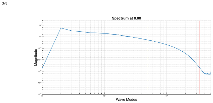
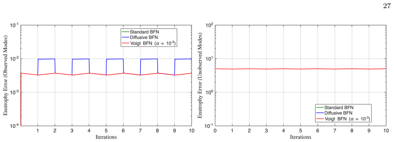
- [VBFN experiments] VBFN comparison for 2D Navier-Stokes: the conclusion that VBFN 'still cannot reconstruct the unobserved fine spatial scales' is load-bearing for the broader claim, yet no spectral decomposition, energy spectrum plot, or explicit comparison of unresolved modes versus the reference solution is given to quantify the residual error.
minor comments (2)
- [Introduction / Preliminaries] The observation operator is used throughout but never given a compact mathematical definition (e.g., as a sum of Dirac deltas or interpolation operator) in the preliminaries; this notation should be fixed early for clarity.
- [Introduction] Several references to prior BFN and AOT papers are cited, but the manuscript would benefit from a short table contrasting the present kernel argument with earlier uniqueness results under denser observations.
Simulated Author's Rebuttal
We thank the referee for the careful and constructive review. The comments highlight opportunities to strengthen the explicitness of our constructions and the quantitative support for our numerical claims. We address each major comment below and will incorporate the suggested clarifications in a revised manuscript.
read point-by-point responses
-
Referee: [Analytical constructions (heat equation)] § on heat-equation construction: the assertion that higher eigenmodes (odd with respect to interior observation points) lie in the kernel and can be superposed while preserving observations is central, yet no explicit non-trivial example is supplied (e.g., a concrete eigenfunction, observation point x0, and verification that the solution satisfies the PDE and matches data for all t). Without this, the claim that the nudging term vanishes identically remains difficult to verify.
Authors: We agree that an explicit, verifiable example would improve clarity. In the revision we will insert a concrete construction for the heat equation on [0,1] with a single interior observation at x0=1/2. The eigenfunctions sin(2kπx) (k=1,2,…) vanish identically at x=1/2, satisfy the homogeneous heat equation, and therefore produce a zero contribution to the nudging term for any choice of coefficients. Superposition with a reference solution yields an infinite family of distinct solutions that share identical observations at x0 for all t while satisfying the PDE. We will explicitly verify the PDE satisfaction and the vanishing of the observation mismatch. revision: yes
-
Referee: [Numerical results] Numerical simulations section: the manuscript states that simulations support the analytical non-uniqueness, but provides neither the precise definition of the discrete observation operator, the time-stepping scheme, nor quantitative error metrics (L2 or pointwise differences between recovered and reference trajectories) in the figures or tables. This weakens the evidential link between analysis and numerics.
Authors: We accept that the numerical section requires additional implementation details to make the link with the analysis fully transparent. The revised manuscript will specify the discrete observation operator (direct sampling at the observation grid points), the time-stepping method (including order and stability constraints), and will augment the figures with quantitative metrics such as L2-norm differences and pointwise errors between the recovered and reference trajectories over the assimilation window. revision: yes
-
Referee: [VBFN experiments] VBFN comparison for 2D Navier-Stokes: the conclusion that VBFN 'still cannot reconstruct the unobserved fine spatial scales' is load-bearing for the broader claim, yet no spectral decomposition, energy spectrum plot, or explicit comparison of unresolved modes versus the reference solution is given to quantify the residual error.
Authors: We agree that a quantitative demonstration of the unresolved scales would strengthen the claim. In the revision we will add an energy-spectrum comparison (log-log plot of kinetic energy versus wavenumber) between the VBFN reconstruction and the reference solution, together with a decomposition of the residual energy into resolved and unresolved modes. This will explicitly document the persistent gap at high wavenumbers. revision: yes
Circularity Check
No significant circularity
full rationale
The paper's central claim rests on explicit constructions of distinct solutions to the heat equation, transport equation, Burgers equations, and Lorenz system that agree on the values of a spatially sparse observation operator for all time. These constructions follow directly from the kernel of the observation map (e.g., higher eigenmodes vanishing at interior points) and the fact that the nudging term depends only on pointwise differences at observed locations; the argument invokes no fitted parameters, no self-referential definitions, and no load-bearing citations to prior work by the same authors. The introduction of VBFN regularization is presented as an auxiliary numerical fix whose limitations are then verified by the same kernel argument, without circular reduction. The derivation chain is therefore self-contained and externally falsifiable by direct substitution into the PDEs.
Axiom & Free-Parameter Ledger
axioms (1)
- domain assumption The systems under study are dissipative and admit solutions that remain indistinguishable under spatially sparse observations.
Reference graph
Works this paper leans on
-
[1]
Samira Amraoui, Didier Auroux, Jacques Blum, and Emmanuel Cosme. Back-and-forth nudging for the quasi-geostrophic ocean dynamics with altimetry: Theoretical convergence study and numerical experiments with the future SWOT observations.Discrete & Continuous Dynamical Systems-Series S, 16(2), 2023
work page 2023
-
[2]
Didier Auroux.Etude de diff´ erentes m´ ethodes d’assimilation de donn´ ees pour l’environnement. PhD thesis, Nice, 2003
work page 2003
-
[3]
Didier Auroux. The back and forth nudging algorithm applied to a shallow water model, compar- ison and hybridization with the 4D-VAR.International Journal for Numerical Methods in Fluids, 61(8):911–929, 2009
work page 2009
-
[4]
Didier Auroux, Patrick Bansart, and Jacques Blum. An evolution of the back and forth nudging for geophysical data assimilation: application to Burgers equation and comparisons.Inverse Problems in Science and Engineering, 21(3):399–419, 2013
work page 2013
-
[5]
Back and forth nudging algorithm for data assimilation problems
Didier Auroux and Jacques Blum. Back and forth nudging algorithm for data assimilation problems. Comptes Rendus. Math´ ematique, 340(12):873–878, 2005
work page 2005
-
[6]
Didier Auroux and Jacques Blum. A nudging-based data assimilation method: the Back and Forth Nudging (BFN) algorithm.Nonlinear Processes in Geophysics, 15(2):305–319, 2008
work page 2008
-
[7]
Data assimilation for geophysical fluids: the diffusive back and forth nudging
Didier Auroux, Jacques Blum, and Giovanni Ruggiero. Data assimilation for geophysical fluids: the diffusive back and forth nudging. InMathematical Paradigms of Climate Science, pages 139–174. Springer, 2016
work page 2016
-
[8]
Didier Auroux and Ma¨ elle Nodet. The back and forth nudging algorithm for data assimilation prob- lems: theoretical results on transport equations.ESAIM: Control, Optimisation and Calculus of Variations, 18(2):318–342, 2012
work page 2012
-
[9]
Abderrahim Azouani, Eric Olson, and Edriss S. Titi. Continuous data assimilation using general interpolant observables.J. Nonlinear Sci., 24(2):277–304, 2014. 33
work page 2014
-
[10]
Abderrahim Azouani and Edriss S. Titi. Feedback control of nonlinear dissipative systems by finite determining parameters—a reaction-diffusion paradigm.Evol. Equ. Control Theory, 3(4):579–594, 2014
work page 2014
-
[11]
T. Brooke Benjamin, Jerry L. Bona, and John J. Mahony. Model equations for long waves in non- linear dispersive systems.Philosophical Transactions of the Royal Society of London. Series A, Mathematical and Physical Sciences, 272(1220):47–78, 1972
work page 1972
-
[12]
Animikh Biswas, Zachary Bradshaw, and Michael Jolly. Convergence of a mobile data assimila- tion scheme for the 2D Navier-Stokes equations.Discrete and Continuous Dynamical Systems, 43(11):4042–4068, 2023
work page 2023
-
[13]
Jordan Blocher, Vincent R Martinez, and Eric Olson. Data assimilation using noisy time-averaged measurements.Physica D: Nonlinear Phenomena, 376:49–59, 2018
work page 2018
- [14]
-
[15]
Yanping Cao, Evelyn M Lunasin, and Edriss S. Titi. Global well-posedness of the three-dimensional viscous and inviscid simplified Bardina turbulence models.Commun. Math. Sci., 4(1):823–848, 2006
work page 2006
-
[16]
Elizabeth Carlson, Aseel Farhat, Vincent R. Martinez, and Collin Victor. On the nudging approach to continuous data assimilation in the limit of infinite error feedback gain.SIAM Journal on Control and Optimization, 2026. (Accepted)
work page 2026
-
[17]
Bernardo Cockburn, Don A. Jones, and Edriss S. Titi. Estimating the number of asymptotic degrees of freedom for nonlinear dissipative systems.Mathematics of Computation, 66(219):1073–1087, 1997
work page 1997
-
[18]
Yi Juan Du and Ming-Cheng Shiue. Analysis and computation of continuous data assimilation algorithms for Lorenz 63 system based on nonlinear nudging techniques.Journal of Computational and Applied Mathematics, 386:113246, 2021
work page 2021
-
[19]
Cambridge University Press, Cambridge, 2001
Ciprian Foias, Oscar Manley, Ricardo Rosa, and Roger Temam.Navier-Stokes Equations and Turbu- lence, volume 83 ofEncyclopedia of Mathematics and its Applications. Cambridge University Press, Cambridge, 2001
work page 2001
-
[20]
Ciprian Foia¸ s and Giovanni Prodi. Sur le comportement global des solutions non-stationnaires des ´ equations de Navier-Stokes en dimension 2.Rendiconti del Seminario Matematico della Universit` a di Padova, 39:1–34, 1967
work page 1967
-
[21]
Ciprian Foia¸ s and Roger Temam. Determination of the solutions of the Navier-Stokes equations by a set of nodal values.Mathematics of Computation, 43(167):117–133, 1984
work page 1984
-
[22]
Ciprian Foia¸ s and Edriss S. Titi. Determining nodes, finite difference schemes and inertial manifolds. Nonlinearity, 4(1):135–153, 1991
work page 1991
-
[23]
Masakazu Gesho, Eric Olson, and Edriss S. Titi. A computational study of a data assimilation algorithm for the two-dimensional Navier–Stokes equations.Commun. Comput. Phys., 19(4):1094– 1110, 2016
work page 2016
-
[24]
PhD thesis, Masters Thesis, University of Nevada, Department of Mathematics and Statistics, 2007
Kevin Hayden.Synchronization in the Lorenz System. PhD thesis, Masters Thesis, University of Nevada, Department of Mathematics and Statistics, 2007
work page 2007
-
[25]
Kevin Hayden, Eric Olson, and Edriss S. Titi. Discrete data assimilation in the Lorenz and 2D Navier–Stokes equations.Phys. D, 240(18):1416–1425, 2011
work page 2011
-
[26]
James E Hoke and Richard A Anthes. The initialization of numerical models by a dynamic- initialization technique.Monthly Weather Review, 104(12):1551–1556, 1976
work page 1976
-
[27]
Michael J. Holst and Edriss S. Titi. Determining projections and functionals for weak solutions of the Navier-Stokes equations. InThe Curth Edwards Memorial Volume, volume 204 ofContemporary Mathematics, pages 125–138. American Mathematical Society, 1997
work page 1997
-
[28]
Jolly, Tural Sadigov, and Edriss S
Michael S. Jolly, Tural Sadigov, and Edriss S. Titi. Determining form and data assimilation algo- rithm for weakly damped and driven Korteweg–de Vries equation—Fourier modes case.Nonlinear Analysis: Real World Applications, 36:287–317, 2017
work page 2017
-
[29]
Don A. Jones and Edriss S. Titi. Determining finite volume elements for the 2D Navier-Stokes equations.Physica D: Nonlinear Phenomena, 60(1–4):165–174, 1992
work page 1992
-
[30]
Don A. Jones and Edriss S. Titi. Upper bounds on the number of determining modes, nodes and vol- ume elements for the Navier-Stokes equations.Indiana University Mathematics Journal, 42(3):875– 887, 1993
work page 1993
-
[31]
Varga K. Kalantarov and Edriss S. Titi. Global attractors and determining modes for the 3D Navier- Stokes-Voigt equations.Chinese Annals of Mathematics, Series B, 30(6):697–714, 2009
work page 2009
- [32]
-
[33]
Analysis of the 3DVAR filter for the partially observed Lorenz ’63 model, 2014
Kody Law, Abhishek Shukla, and Andrew Stuart. Analysis of the 3DVAR filter for the partially observed Lorenz ’63 model, 2014
work page 2014
-
[34]
Boris Levant, F´ abio Ramos, and Edriss S. Titi. On the statistical properties of the 3D incompressible Navier-Stokes-Voigt model.Communications in Mathematical Sciences, 8(1):277–293, 2010
work page 2010
-
[35]
Deterministic nonperiodic flow.Journal of atmospheric sciences, 20(2):130–141, 1963
Edward N Lorenz. Deterministic nonperiodic flow.Journal of atmospheric sciences, 20(2):130–141, 1963. 34
work page 1963
-
[36]
Almudena P M´ arquez and Mar´ ıa S Bruz´ on. Symmetry analysis and conservation laws of a general- ization of the Kelvin-Voigt viscoelasticity equation.Symmetry, 11(7):840, 2019
work page 2019
-
[37]
Eric Olson and Edriss S. Titi. Determining modes for continuous data assimilation in 2D turbulence. J. Statist. Phys., 113(5-6):799–840, 2003. Progress in statistical hydrodynamics (Santa Fe, NM, 2002)
work page 2003
-
[38]
Anatolii Petrovich Oskolkov. The uniqueness and solvability in the large of boundary value problems for the equations of motion of aqueous solutions of polymers.Zap. Nauchn. Sem. Leningrad. Otdel. Mat. Inst. Steklov. (LOMI), 38:98–136, 1973
work page 1973
-
[39]
Synchronization in chaotic systems.Physical review letters, 64(8):821, 1990
Louis M Pecora and Thomas L Carroll. Synchronization in chaotic systems.Physical review letters, 64(8):821, 1990
work page 1990
-
[40]
Yu Chen Peng, Liang Chun Wu, and Ming-Cheng Shiue. Finite time synchronization of the continu- ous/discrete data assimilation algorithms for Lorenz 63 system based on the back and forth nudging techniques.Results in Applied Mathematics, 20:100407, 2023
work page 2023
-
[41]
Springer Science & Business Media, 2013
Roger Peyret.Spectral Methods for Incompressible Viscous Flow, volume 148. Springer Science & Business Media, 2013
work page 2013
-
[42]
Fabio Ramos and Edriss S. Titi. Invariant measures for the 3D Navier–Stokes-Voigt equations and their Navier–Stokes limit.Discrete Contin. Dyn. Syst., 28(1):375–403, 2010
work page 2010
-
[43]
Jie Shen, Tao Tang, and Li-Lian Wang.Spectral Methods, volume 41 ofSpringer Series in Compu- tational Mathematics. Springer, Heidelberg, 2011. Algorithms, analysis and applications
work page 2011
-
[44]
Springer-Verlag, New York, second edition, 1997
Roger Temam.Infinite-Dimensional Dynamical Systems In Mechanics and Physics, volume 68 of Applied Mathematical Sciences. Springer-Verlag, New York, second edition, 1997
work page 1997
-
[45]
Edriss S. Titi and Collin Victor. On the inadequacy of nudging data assimilation algorithms for non-dissipative systems.Discrete and Continuous Dynamical Systems - S, 2025
work page 2025
-
[46]
Trefethen.Spectral Methods in MATLAB, volume 10 ofSoftware, Environments, and Tools
Lloyd N. Trefethen.Spectral Methods in MATLAB, volume 10 ofSoftware, Environments, and Tools. Society for Industrial and Applied Mathematics (SIAM), Philadelphia, PA, 2000
work page 2000
-
[47]
Warwick Tucker. The Lorenz attractor exists.Comptes Rendus de l’Acad´ emie des Sciences - Series I - Mathematics, 328(12):1197–1202, 1999. (Aseel F arhat) Department of Mathematics, University of Virginia, Charlottesville, V A 22904, USA Email address:af7py@virginia.edu (Edriss S. Titi) Department of Applied Mathematics and Theoretical Physics, University...
work page 1999
discussion (0)
Sign in with ORCID, Apple, or X to comment. Anyone can read and Pith papers without signing in.