A mixed interpolation-regression method for numerical integration on some planar domains
Pith reviewed 2026-05-08 01:56 UTC · model grok-4.3
The pith
A mixed interpolation-regression operator is introduced for functions on ellipses, annuli, and polygons, yielding an upper bound and cubature formulas.
A machine-rendered reading of the paper's core claim, the machinery that carries it, and where it could break.
Core claim
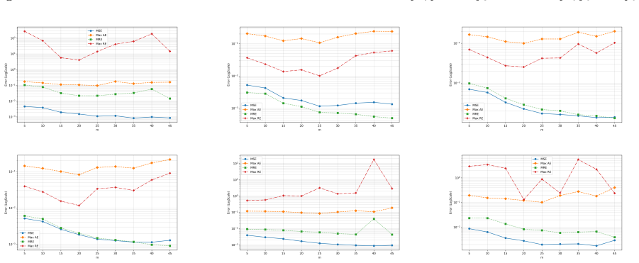
We introduce a mixed interpolation-regression operator for functions defined in some domains of the plane. We focus the attention on the ellipse, an annulus and a polygon. An upper bound for such an operator is obtained. Cubature formulas for weight functions defined in such domains are studied. The performance of the above interpolation-regression methods is illustrated with some numerical examples taking into account the variations of the dimension of the interpolation and the regression part, respectively.
What carries the argument
The mixed interpolation-regression operator that blends interpolation at selected points with regression over a set of points to approximate functions and support cubature rules on planar domains.
If this is right
- The upper bound on the operator allows for error estimates in function approximation on the given domains.
- Cubature formulas enable the numerical evaluation of integrals with respect to weight functions on the ellipse, annulus, and polygon.
- Varying the relative sizes of the interpolation and regression parts permits optimization of the method's accuracy as demonstrated in examples.
- The approach extends standard interpolation by incorporating a regression component for potentially improved stability or accuracy.
Where Pith is reading between the lines
- This mixed approach could be adapted to other two-dimensional domains beyond the three studied here.
- Connections to existing cubature rules in numerical analysis might lead to hybrid methods with better convergence properties.
- Practical implementations could benefit from automated selection of interpolation and regression dimensions based on function properties.
Load-bearing premise
The upper bound for the mixed operator holds under the specific choices of domains, points, and weight functions considered in the study.
What would settle it
A direct computation of the operator's norm on the ellipse domain that exceeds the provided upper bound for a particular choice of interpolation and regression dimensions.
Figures




read the original abstract
In this contribution we introduce a mixed interpolation-regression operator for functions defined in some domains of the plane. We focus the attention on the ellipse, an annulus and a polygon. An upper bound for such an operator is obtained. Cubature formulas for weight functions defined in such domains are studied. The performance of the above interpolation-regression methods is illustrated with some numerical examples taking into account the variations of the dimension of the interpolation and the regression part, respectively.
Editorial analysis
A structured set of objections, weighed in public.
Referee Report
Summary. The paper introduces a mixed interpolation-regression operator for functions defined on the ellipse, annulus, and polygon domains in the plane. It derives an upper bound for this operator and uses the construction to study cubature formulas for weight functions on the same domains. Numerical examples are presented that vary the respective dimensions of the interpolation and regression components to illustrate performance.
Significance. If the upper bound is rigorously established under appropriate hypotheses and the resulting cubature formulas are accurate, the mixed operator could supply a flexible approximation tool for numerical integration on non-standard planar domains. The combination of interpolation and regression is a potentially useful idea, but the absence of explicit comparisons with existing methods (e.g., Gaussian or other polynomial-based cubatures) and of concrete error estimates limits the immediate significance to a preliminary methodological contribution.
major comments (2)
- [Section defining the mixed operator and its upper bound] The statement of the upper bound for the mixed interpolation-regression operator (appearing after the definition of the operator) does not specify the underlying function space or the norm in which the bound holds. For the bound to control quadrature error for general weight functions, it must be stated in a concrete norm (uniform, L^2, etc.) and for a concrete smoothness class (C^k, Sobolev, etc.). Without these hypotheses the claimed applicability to the advertised weight functions cannot be verified.
- [Sections on the upper bound and on the cubature formulas] No derivation of the upper bound or error analysis linking the operator bound to the cubature error is supplied. The central claim that the mixed operator yields usable cubature formulas therefore rests on an unproven step; an explicit proof or reference to a standard approximation-theory result under stated assumptions is required.
minor comments (2)
- [Abstract] The abstract would be clearer if it indicated the precise norm and function class for the upper bound and mentioned whether the numerical examples include any baseline comparisons.
- [Section introducing the operator] Notation for the mixed operator (interpolation part versus regression part) should be introduced with an explicit formula or diagram at first use to aid readability.
Simulated Author's Rebuttal
We thank the referee for the careful reading of our manuscript and for identifying points where additional rigor is needed in the presentation of the theoretical results. We address each major comment below and will incorporate the necessary clarifications and proofs in the revised version.
read point-by-point responses
-
Referee: [Section defining the mixed operator and its upper bound] The statement of the upper bound for the mixed interpolation-regression operator (appearing after the definition of the operator) does not specify the underlying function space or the norm in which the bound holds. For the bound to control quadrature error for general weight functions, it must be stated in a concrete norm (uniform, L^2, etc.) and for a concrete smoothness class (C^k, Sobolev, etc.). Without these hypotheses the claimed applicability to the advertised weight functions cannot be verified.
Authors: We agree that the hypotheses for the operator bound must be stated explicitly. The bound is intended to hold in the uniform norm on the space C(D) of continuous functions on the compact domain D (ellipse, annulus, or polygon). We will revise the manuscript to state this clearly, including that the weight functions are assumed continuous on D to ensure the cubature error is controlled by the operator norm. revision: yes
-
Referee: [Sections on the upper bound and on the cubature formulas] No derivation of the upper bound or error analysis linking the operator bound to the cubature error is supplied. The central claim that the mixed operator yields usable cubature formulas therefore rests on an unproven step; an explicit proof or reference to a standard approximation-theory result under stated assumptions is required.
Authors: We acknowledge that the derivation of the upper bound and the link to cubature error were not provided in sufficient detail. The bound is obtained by combining standard estimates for the interpolation and regression components in the uniform norm, and the cubature error follows from the usual representation of the quadrature remainder via the operator. We will add a complete, self-contained proof of the operator-norm bound together with the explicit error estimate for the cubature formulas in the revised manuscript. revision: yes
Circularity Check
No circularity: operator and bound derived from standard approximation theory
full rationale
The paper introduces a mixed interpolation-regression operator on ellipse/annulus/polygon domains, derives an upper bound for the operator, and applies it to cubature formulas for given weight functions. No equations or steps in the provided abstract reduce the claimed bound or formulas to a fitted parameter, self-definition, or self-citation chain; the construction is presented as a direct application of interpolation-regression techniques without tautological renaming or input-as-prediction. The reader's assessment of score 2.0 aligns with absence of load-bearing circularity, and the skeptic concern addresses missing hypotheses rather than derivation circularity.
Axiom & Free-Parameter Ledger
Reference graph
Works this paper leans on
-
[1]
Delgado, and Lidia Fern´ andez
Sergio Barbero, Antonia M. Delgado, and Lidia Fern´ andez. An explanation of the number or points and symmetries of starbursts, 2025
work page 2025
-
[2]
Society for Industrial and Applied Mathe- matics, Philadelphia, PA, 1996
˚Ake Bj¨ orck.Numerical Methods for Least Squares Problems. Society for Industrial and Applied Mathe- matics, Philadelphia, PA, 1996
work page 1996
-
[3]
On polynomial interpolation of two variables.Journal of Approximation Theory, 120(2):267–282, 2003
Borislav Bojanov and Yuan Xu. On polynomial interpolation of two variables.Journal of Approximation Theory, 120(2):267–282, 2003
work page 2003
-
[4]
Stefano De Marchi, Francesco Dell’Accio, and Mariarosa Mazza. On the constrained mock-Chebyshev least-squares.Journal of Computational and Applied Mathematics, 280:94–109, 2015. 24
work page 2015
-
[5]
Constrained mock-Chebyshev least squares quadrature.Applied Mathematics Letters, 134:108328, 2022
Francesco Dell’Accio, Filomena Di Tommaso, and Federico Nudo. Constrained mock-Chebyshev least squares quadrature.Applied Mathematics Letters, 134:108328, 2022
work page 2022
-
[6]
Francesco Dell’Accio, Francisco Marcell´ an, and Federico Nudo. Constrained mock-Chebyshev least squares approximation for Hermite interpolation.Numerical Algorithms, In press, 2026
work page 2026
-
[7]
Francesco dell’Accio, Domenico Mezanotte, Federico Nudo, and Donatella Occorsio. Numerical approxi- mation of Fredholm integral equation by the constrained mock-Chebyshev least squares operator.Journal of Computational and Applied Mathematics, 447:115886, 2024
work page 2024
-
[8]
Francesco dell’Accio and Federico Nudo. Polynomial approximation of derivatives through a regression- interpolation method.Applied Mathematics Letters, 152:109010, 2024
work page 2024
-
[9]
Francesco Dell’Accio, Filomena Di Tommaso, and Federico Nudo. Generalizations of the constrained mock- Chebyshev least squares in two variables: Tensor product vs total degree polynomial interpolation.Applied Mathematics Letters, 125:107732, 2022
work page 2022
-
[10]
Francesco Dell’Accio, Francisco Marcell´ an, and Federico Nudo. An extension of a mixed interpola- tion–regression method using zeros of orthogonal polynomials.Journal of Computational and Applied Mathematics, 450:116010, 2024
work page 2024
-
[11]
Francesco Dell’Accio, Francisco Marcell´ an, and Federico Nudo. An interpolation–regression approach for function approximation on the disk and its application to cubature formulas.Advances in Computational Mathematics, 51:53, 2025
work page 2025
-
[12]
Charles F. Dunkl and Yuan Xu.Orthogonal Polynomials of Several Variables, Second Edition, volume 155 ofEncyclopedia of Mathematics and its Applications. Cambridge University Press, Cambridge, 2014
work page 2014
-
[13]
Sergio D´ ıaz-Elbal, Andrei Mart´ ınez-Finkelshtein, and Dar´ ıo Ramos-L´ opez. Sampling patterns for Zernike- like bases in non-standard geometries.Applied Mathematics and Computation, 511:129727, 2026
work page 2026
-
[14]
L´ opez, Rafael Navarro, and Ester P´ erez Sinus´ ıa
Chelo Ferreira, Jos´ e L. L´ opez, Rafael Navarro, and Ester P´ erez Sinus´ ıa. Zernike-like systems in polygons and polygonal facets.Applied Optics, 54(21):6575–6583, Jul 2015
work page 2015
-
[15]
Stefano De Marchi, Francesco Dell’Accio, and Federico Nudo. A mixed interpolation-regression approxi- mation operator on the triangle.Dolomites Research Notes on Approximation, 17:33–44, 2024
work page 2024
-
[16]
Andrei Mart´ ınez-Finkelshtein, Antonia M. Delgado, Gracia M. Castro, Alejandro Zarzo, and Jorge L. Ali´ o. Comparative analysis of some modal reconstruction methods of the shape of the cornea from corneal elevation data.Investigative Ophthalmology & Visual Science, 50(12):5639–5645, 2009
work page 2009
-
[17]
Rafael Navarro, Jos´ e L. L´ opez, Jos´ e A. D´ ıaz, and Ester P´ erez Sinus´ ıa. Generalization of Zernike polynomials for regular portions of circles and ellipses and their applications.Optics Express, 22(18):21263–21279, Sept 2014
work page 2014
-
[18]
Zernike polynomials and their applications.Journal of Optics, 24:123001, 2022
Kuo Niu and Chao Tian. Zernike polynomials and their applications.Journal of Optics, 24:123001, 2022
work page 2022
-
[19]
S´ anchez-Granero, Manuel Fern´ andez-Mart´ ınez, and Andrei Mart´ ınez–Finkelshtein
Dar´ ıo Ramos-L´ opez, Miguel A. S´ anchez-Granero, Manuel Fern´ andez-Mart´ ınez, and Andrei Mart´ ınez–Finkelshtein. Optimal sampling patterns for Zernike polynomials.Applied Mathematics and Computation, 274:247–257, 2016
work page 2016
-
[20]
https://sites.google.com/view/alvisesommarivaunipd/home-page/sets, 2026
Alvise Sommariva. https://sites.google.com/view/alvisesommarivaunipd/home-page/sets, 2026
work page 2026
-
[21]
American Mathematical Society, Providence, RI, 1975
G´ abor Szeg¨ o.Orthogonal Polynomials, Fourth Edition, volume 23 ofAmerican Mathematical Society Colloquium Publications. American Mathematical Society, Providence, RI, 1975
work page 1975
-
[22]
Frits Zernike and Frederick J. M. Stratton. Diffraction Theory of the Knife-Edge Test and its Improved Form, The Phase-Contrast Method.Monthly Notices of the Royal Astronomical Society, 94(5):377–384, March 1934. eprint: https://academic.oup.com/mnras/article-pdf/94/5/377/3785471/mnras94-0377.pdf. 25
work page 1934
discussion (0)
Sign in with ORCID, Apple, or X to comment. Anyone can read and Pith papers without signing in.