Testing linear combinations of multiple variance components
Pith reviewed 2026-05-07 15:17 UTC · model grok-4.3
The pith
A parametric bootstrap procedure tests simultaneous linear contrasts of multiple variance components equaling zero in Gaussian models.
A machine-rendered reading of the paper's core claim, the machinery that carries it, and where it could break.
Core claim
We test the hypothesis that simultaneous linear contrasts of multiple variance components equal zero in a Gaussian variance components model via a parametric bootstrap. The main technical contributions are a computationally efficient decomposition of the normalized residual log-likelihood that does not require the variance components to be non-negative or variance design matrices to be positive semi-definite, a modified Newton method for its minimization, and a method for efficient optimization and sampling under the null hypothesis that certain linear combinations of variance components equal zero. A special case of the proposed procedure is a test for multiple variance components simulatne
What carries the argument
Parametric bootstrap test for linear contrasts of variance components, enabled by an efficient decomposition of the normalized residual log-likelihood that avoids non-negativity and positive semi-definiteness constraints.
Load-bearing premise
The observations follow a Gaussian variance components model and the parametric bootstrap accurately approximates the null distribution of the test statistic for the linear contrasts.
What would settle it
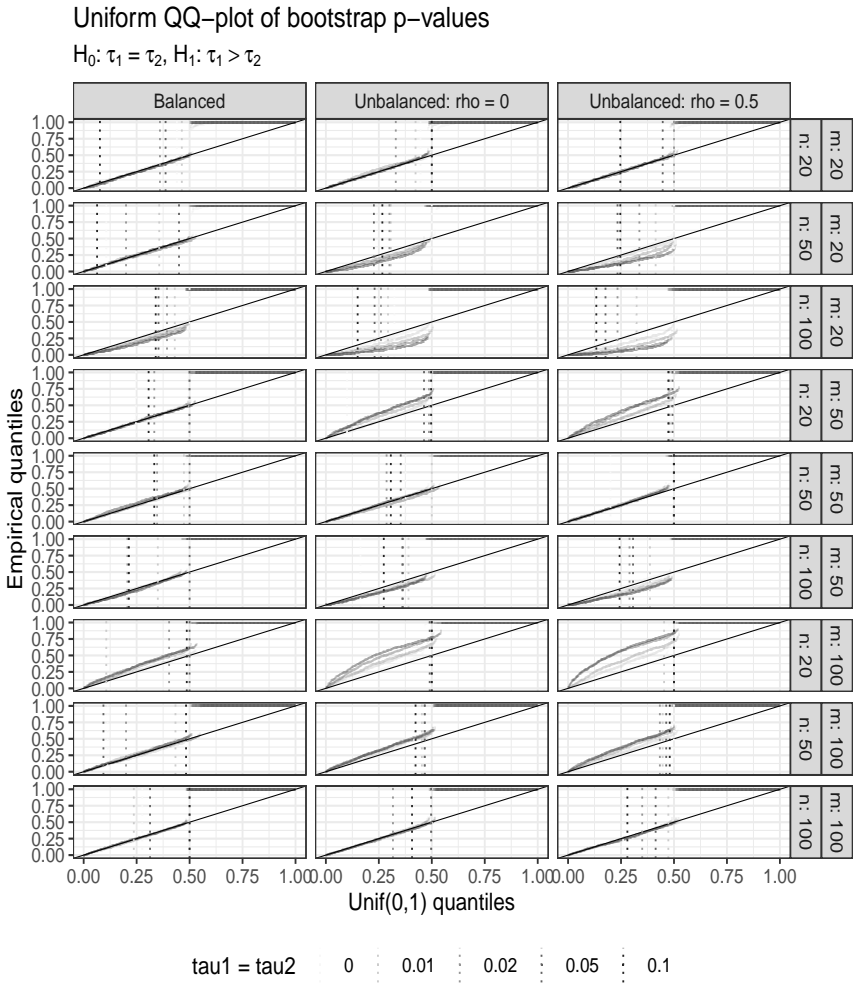
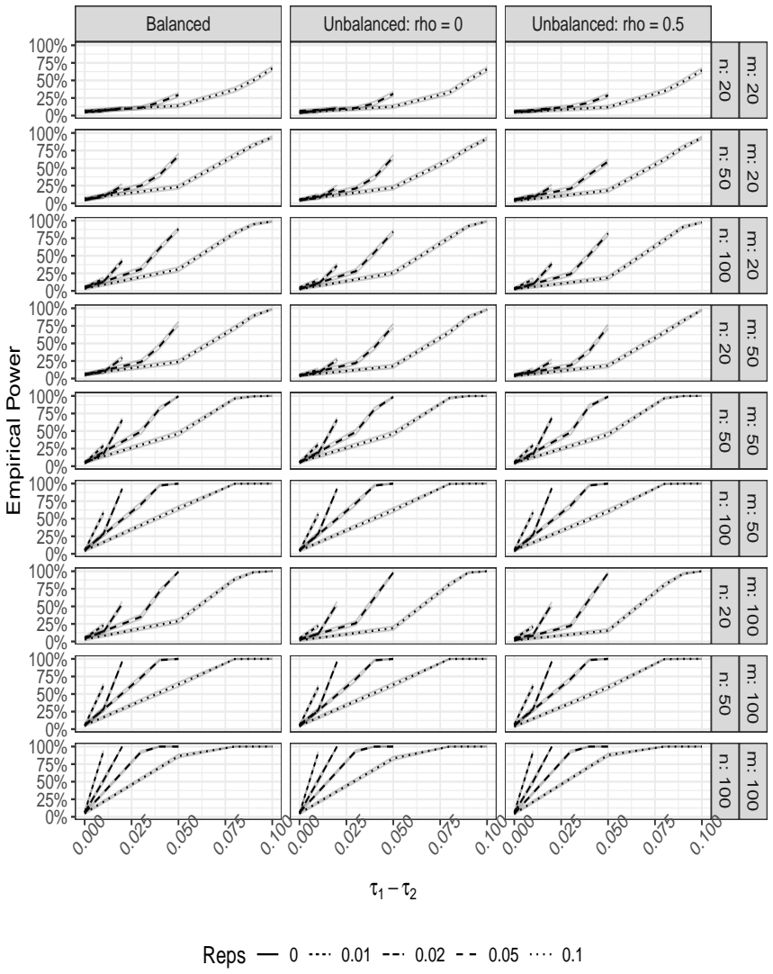
A simulation study in which the test rejects the null at rates substantially different from the nominal significance level when the null is true would show the bootstrap approximation fails.
Figures


read the original abstract
We test the hypothesis that simulataneous linear contrasts of multiple variance components equal zero in a Gaussian variance components model via a parametric bootstrap. Applications include but are not limited to nested and crossed designs. The main technical contributions are a computationally efficient decomposition of the normalized residual log-likelihood that does not require the variance components to be non-negative or variance design matrices to be positive semi-definite, a modified Newton method for its minimization, and a method for efficient optimization and sampling under the null hypothesis that certain linear combinations of variance components equal zero. A special case of the proposed procedure is a test for multiple variance components simulataneously equalling zero, for which a likelihood ratio test was not previously available. However, the proposed procedure is significantly more general.
Editorial analysis
A structured set of objections, weighed in public.
Referee Report
Summary. The manuscript proposes a parametric bootstrap procedure for testing hypotheses that linear combinations of multiple variance components equal zero in a Gaussian variance components model. Central technical contributions include a computationally efficient decomposition of the normalized residual log-likelihood that does not require non-negative variance components or positive semi-definite design matrices, a modified Newton method for its minimization, and methods for efficient optimization and sampling under the null. A highlighted special case is simultaneous testing of multiple variance components equaling zero, for which a likelihood ratio test was previously unavailable; the procedure is presented as more general and applicable to nested and crossed designs.
Significance. If the core procedure is valid, the work would provide a useful general tool for hypothesis testing on linear contrasts of variance components in linear mixed models, extending beyond existing methods limited to individual components or specific designs. The claimed computational efficiency, avoidance of non-negativity constraints, and availability of a test where LRT was unavailable are potential strengths for practical applications in statistics.
major comments (1)
- [Abstract] Abstract and method description: the central claim that the decomposition of the normalized residual log-likelihood does not require non-negative variance components or positive semi-definite design matrices G_i conflicts with the requirements of the Gaussian model. For the log-likelihood (log det(V) and quadratic form) to be defined over the reals, V = sum theta_i G_i must remain positive semi-definite. If the decomposition permits regions with negative eigenvalues, the objective function, Newton minimization, and parametric bootstrap samples under the linear null become ill-posed. This is load-bearing for both the special-case test of multiple components equaling zero and the general linear-contrast tests, and requires explicit clarification or safeguards.
minor comments (2)
- [Abstract] Typo: 'simulataneous' should be 'simultaneous'.
- [Abstract] Typo: 'simulataneously' should be 'simultaneously'.
Simulated Author's Rebuttal
We thank the referee for their careful reading and for raising this important point concerning the domain of the log-likelihood. We address the major comment below.
read point-by-point responses
-
Referee: [Abstract] Abstract and method description: the central claim that the decomposition of the normalized residual log-likelihood does not require non-negative variance components or positive semi-definite design matrices G_i conflicts with the requirements of the Gaussian model. For the log-likelihood (log det(V) and quadratic form) to be defined over the reals, V = sum theta_i G_i must remain positive semi-definite. If the decomposition permits regions with negative eigenvalues, the objective function, Newton minimization, and parametric bootstrap samples under the linear null become ill-posed. This is load-bearing for both the special-case test of multiple components equaling zero and the general linear-contrast tests, and requires explicit clarification or safeguards.
Authors: We agree that the Gaussian log-likelihood is defined only when V = sum theta_i G_i is positive semi-definite. The decomposition itself is an exact algebraic identity for the normalized residual log-likelihood that can be written without embedding non-negativity of the theta_i or positive semi-definiteness of the individual G_i into the formula. This is the sense in which the decomposition does not require those conditions. In all numerical work, however, the modified Newton minimization and the parametric bootstrap are restricted to the region where V is positive semi-definite; this is enforced by the line-search and by sampling only from valid null distributions. We will revise the abstract and the relevant methodological sections to state this domain restriction explicitly and to describe the safeguards that prevent evaluation at points with negative eigenvalues. The revision will cover both the general linear-contrast tests and the special case of simultaneous zero tests. revision: yes
Circularity Check
No circularity: derivation relies on standard likelihood decomposition and external parametric bootstrap simulation
full rationale
The paper derives a decomposition of the normalized residual log-likelihood for Gaussian variance components models, a modified Newton optimizer, and a parametric bootstrap for testing linear contrasts under the null. These steps are constructed from first-principles matrix algebra and simulation from the fitted null model rather than reducing to fitted parameters by construction or self-citation chains. The bootstrap approximates the null distribution via independent draws, not by renaming or smuggling inputs. No self-definitional equivalences, fitted-input predictions, or load-bearing self-citations appear in the central claims. The special-case test for multiple components equaling zero follows directly as an instance of the general linear-contrast procedure without circular reduction.
Axiom & Free-Parameter Ledger
axioms (1)
- domain assumption Data follows a Gaussian variance components model
Reference graph
Works this paper leans on
-
[1]
Bates, D., Maechler, M., Bolker, B., and Walker, S. (2015). Fitting linear mixed-effects models using lme4.Journal of Statistical Software, 67(1):1–48. Battey, H. and McCullagh, P. (2024). An anomaly arising in the analysis of processes with more than one source of variability.Biometrika, 111(2):677–689. Bezanson, J., Edelman, A., Karpinski, S., and Shah,...
work page 2015
-
[2]
R Foun- dation for Statistical Computing, Vienna, Austria
R Core Team (2024).R: A Language and Environment for Statistical Computing. R Foun- dation for Statistical Computing, Vienna, Austria. Stram, D. O. and Lee, J. W. (1994). Variance components testing in the longitudinal mixed effects model.Biometrics, pages 1171–1177. Venables, W. N. and Ripley, B. D. (2002). Random and mixed effects. InModern applied stat...
work page 2024
-
[3]
Yates, F. (1935). Complex experiments.Supplement to the Journal of the Royal Statistical Society, 2(2):181–247. Zhang, Y., Ekvall, K. O., and Molstad, A. J. (2025). Fast and reliable confidence intervals for a variance component.Biometrika, 112(2):asaf010. 42
work page 1935
discussion (0)
Sign in with ORCID, Apple, or X to comment. Anyone can read and Pith papers without signing in.