A formal approach to variable selection in difference-in-differences
Pith reviewed 2026-05-09 18:27 UTC · model grok-4.3
The pith
Graphical criteria identify the minimal covariates needed to justify conditional parallel trends in difference-in-differences.
A machine-rendered reading of the paper's core claim, the machinery that carries it, and where it could break.
Core claim
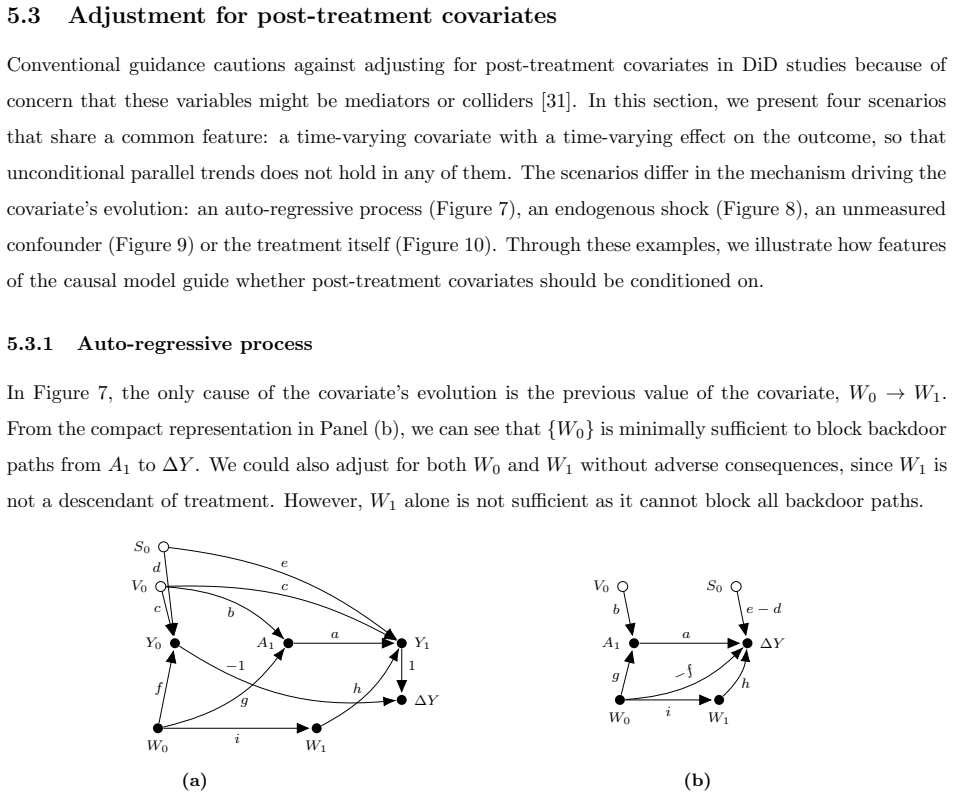
We propose a formal approach to select the variables that support conditional parallel trends based on graphical criteria. We show that the parallel trends assumption is rarely justified without conditioning on covariates, and that unconditional and conditional parallel trends can conflict with one another. We also demonstrate that a time-invariant covariate with a time-invariant effect on the outcome, which might not ordinarily be considered a confounder in DiD, may be a useful conditioning variable. We clarify that adjustment for a post-treatment covariate depends on what causes that covariate to change. Extending our framework to multiple time periods, we distinguish between treatment and
What carries the argument
Directed acyclic graph (DAG) of the data-generating process, with d-separation and backdoor criteria to determine the minimal adjustment set for conditional parallel trends.
If this is right
- Parallel trends rarely holds unconditionally, so covariate adjustment is typically required.
- Unconditional and conditional parallel trends assumptions can contradict each other.
- Time-invariant covariates can still be necessary for identification even if they have time-invariant effects.
- Post-treatment covariates require careful consideration based on their causes.
- Estimation procedures must match the identification adjustment set to avoid bias.
Where Pith is reading between the lines
- Researchers could apply this method to existing DiD studies to check if their chosen covariates are sufficient or minimal.
- This graphical approach might extend to other identifying assumptions in panel data methods beyond DiD.
- The alignment of identification and estimation sets could improve robustness in applied work using popular DiD estimators.
- Testing the sensitivity to different assumed DAGs would be a useful extension for practitioners.
Load-bearing premise
The underlying causal structure among all relevant variables can be correctly represented as a directed acyclic graph.
What would settle it
A real-world DiD application where the graphically selected covariates are adjusted for but the conditional parallel trends assumption is violated, or where the assumption holds without the selected covariates.
Figures


read the original abstract
Difference-in-differences (DiD) identification relies mainly on a parallel trends assumption about untreated potential outcomes. Researchers often relax this assumption by assuming conditional parallel trends within units with the same covariate values. However, the process of selecting which covariates to include in this assumption is often \emph{ad hoc}. We propose a formal approach to select the variables that support conditional parallel trends based on graphical criteria. We show that the parallel trends assumption is rarely justified without conditioning on covariates, and that unconditional and conditional parallel trends can conflict with one another. We also demonstrate that a time-invariant covariate with a time-invariant effect on the outcome, which might not ordinarily be considered a confounder in DiD, may be a useful conditioning variable. We clarify that adjustment for a post-treatment covariate depends on what causes that covariate to change. Extending our framework to multiple time periods, we distinguish between treatment type and rollout strategy and examine the problem of treatment-confounder feedback. On the estimation side, we argue that the difficulty of incorporating covariates in DiD, often framed as an estimator problem, is more accurately understood as a misalignment between the adjustment set used by the estimator and the adjustment set required for identification. This misalignment affects several popular estimation procedures, and resolving it requires not a change of estimator, but a change in how covariates enter the estimation procedure. We show how to achieve this alignment for all estimators we evaluate.
Editorial analysis
A structured set of objections, weighed in public.
Referee Report
Summary. The manuscript proposes a formal graphical approach, based on directed acyclic graphs and d-separation, for selecting the minimal set of covariates that justify a conditional parallel trends assumption in difference-in-differences designs. It argues that unconditional parallel trends is rarely justified without covariates, that unconditional and conditional parallel trends can conflict, that time-invariant covariates with time-invariant effects can be useful conditioning variables, that post-treatment covariate adjustment depends on the causes of change in the covariate, and extends the framework to multiple periods while distinguishing treatment type from rollout strategy and addressing treatment-confounder feedback. On the estimation side, it reframes difficulties with covariates as misalignment between the identification adjustment set and the estimator's adjustment set, and shows how to achieve alignment for the estimators considered.
Significance. If the graphical criteria are shown to correctly encode and imply the counterfactual equality required by conditional parallel trends, the paper would provide a principled, non-ad-hoc method for covariate selection in DiD that could improve identification transparency and validity in applied work. The multi-period extensions and the reframing of estimation issues as alignment problems rather than estimator choice are practically relevant contributions that could influence how researchers specify and implement DiD models.
major comments (3)
- [§3] §3 (graphical criteria for conditional parallel trends): the central claim that d-separation on the proposed DAG identifies the minimal adjustment set supporting conditional parallel trends requires an explicit derivation showing how the graph encodes the counterfactual processes E[Y(0)_t | X, G] and the no-anticipation assumption; without this, standard d-separation on observed variables does not automatically guarantee the required equality of expected untreated potential outcomes across groups.
- [§4.2] §4.2 (conflict between unconditional and conditional PT): the demonstration that these two assumptions can conflict is load-bearing for the motivation to use graphical selection; a concrete counter-example or theorem (with the specific DAG and potential-outcome equations) is needed to show when the conflict arises and whether the proposed minimal adjustment set resolves it without additional parametric restrictions.
- [§6] §6 (multi-period extension and treatment-confounder feedback): the distinction between treatment type and rollout strategy is important, but the graphical criterion for handling feedback must be shown to preserve identification of the target parameter; if the feedback loop is not fully blocked by the selected covariates, the conditional PT may fail in later periods.
minor comments (2)
- The abstract states that 'adjustment for a post-treatment covariate depends on what causes that covariate to change,' but the main text should include a small table or figure contrasting the two cases (e.g., covariate change caused by treatment vs. by an exogenous factor) to improve clarity.
- Notation for potential outcomes and time indices is introduced gradually; a single consolidated notation table at the beginning of §2 would help readers track the distinction between observed and counterfactual quantities.
Simulated Author's Rebuttal
We thank the referee for their constructive and detailed comments, which identify opportunities to strengthen the rigor of our graphical framework for covariate selection in difference-in-differences. We address each major comment below and outline the revisions we will undertake.
read point-by-point responses
-
Referee: [§3] §3 (graphical criteria for conditional parallel trends): the central claim that d-separation on the proposed DAG identifies the minimal adjustment set supporting conditional parallel trends requires an explicit derivation showing how the graph encodes the counterfactual processes E[Y(0)_t | X, G] and the no-anticipation assumption; without this, standard d-separation on observed variables does not automatically guarantee the required equality of expected untreated potential outcomes across groups.
Authors: We agree that an explicit derivation is required to link d-separation directly to the counterfactual equality E[Y(0)_t | X, G] under the no-anticipation assumption. In the revised manuscript we will add a dedicated subsection (or appendix) that derives this connection step by step: we will specify how the DAG encodes the potential-outcome processes, show that the no-anticipation assumption corresponds to the absence of certain directed paths, and prove that d-separation on the minimal adjustment set implies the required conditional independence of untreated potential outcomes across groups. revision: yes
-
Referee: [§4.2] §4.2 (conflict between unconditional and conditional PT): the demonstration that these two assumptions can conflict is load-bearing for the motivation to use graphical selection; a concrete counter-example or theorem (with the specific DAG and potential-outcome equations) is needed to show when the conflict arises and whether the proposed minimal adjustment set resolves it without additional parametric restrictions.
Authors: We acknowledge the need for a fully specified counter-example. The revision will include a concrete DAG together with the associated potential-outcome equations that exhibit a conflict between unconditional and conditional parallel trends. We will then apply our graphical criterion to recover the minimal adjustment set and verify that it restores identification of the target parameter without imposing extra parametric restrictions beyond those already stated in the paper. revision: yes
-
Referee: [§6] §6 (multi-period extension and treatment-confounder feedback): the distinction between treatment type and rollout strategy is important, but the graphical criterion for handling feedback must be shown to preserve identification of the target parameter; if the feedback loop is not fully blocked by the selected covariates, the conditional PT may fail in later periods.
Authors: We agree that preservation of identification must be shown explicitly when treatment-confounder feedback is present. In the revised Section 6 we will provide a formal argument (supported by path-blocking analysis) demonstrating that the covariates selected by our graphical criterion close all feedback paths that would otherwise violate conditional parallel trends in subsequent periods. We will also add a brief numerical illustration confirming that the target parameter remains identified under the proposed adjustment set. revision: yes
Circularity Check
No circularity: standard graphical criteria applied to DiD identification
full rationale
The paper's derivation applies established d-separation and adjustment-set criteria from graphical causal models to the conditional parallel trends assumption in DiD. This is an extension of existing tools rather than a self-referential construction; the parallel trends statement is not redefined in terms of the selected covariates, no parameters are fitted to the target result and then relabeled as predictions, and no load-bearing uniqueness theorems or ansatzes are imported solely via self-citation. The central claim remains an independent mapping from DAG structure to covariate sets, with the identification result following from the graphical rules rather than reducing to the paper's own inputs by construction.
Axiom & Free-Parameter Ledger
axioms (2)
- standard math Causal relationships among variables can be represented by a directed acyclic graph (DAG).
- domain assumption The (conditional) parallel trends assumption corresponds to specific conditional independence relations in the DAG.
Reference graph
Works this paper leans on
-
[1]
The Estimation of Causal Effects by Difference-in-Difference Methods
Lechner M. The Estimation of Causal Effects by Difference-in-Difference Methods. Foundations and Trends in Econometrics. 2011;4(3):165-224
work page 2011
-
[2]
What’s Trending in Difference-in-Differences? A Synthesis of the Recent Econometrics Literature
Roth J, Sant’Anna PHC, Bilinski A, Poe J. What’s Trending in Difference-in-Differences? A Synthesis of the Recent Econometrics Literature. Journal of Econometrics. 2023;235(2):2218-44
work page 2023
-
[3]
Bilinski A, Hatfield LA. Nothing to See Here? A non-inferiority approach to evaluation of parallel trends in difference-in-differences. Statistics in Medicine. 2026 Feb;45(3-5)
work page 2026
-
[4]
Semiparametric Difference-in-Differences Estimators
Abadie A. Semiparametric Difference-in-Differences Estimators. Review of Economic Studies. 2005;72:1- 19
work page 2005
-
[5]
Confounding and Regression Adjustment in Difference-in-Differences Studies
Zeldow B, Hatfield LA. Confounding and Regression Adjustment in Difference-in-Differences Studies. Health Services Research. 2021;56:932-41
work page 2021
-
[6]
Causality: Models, Reasoning, and Inference
Pearl J. Causality: Models, Reasoning, and Inference. 2nd ed. New York: Cambridge University Press; 2000
work page 2000
-
[7]
Causal Inference in Statistics: A Primer
Pearl J, Glymour M, Jewell NP. Causal Inference in Statistics: A Primer. Chichester, West Sussex: Wiley; 2016
work page 2016
-
[8]
Hern´ an MA, Hern´ andez-D´ ıaz S, Werler MM, Mitchell AA. Causal Knowledge as a Prerequisite for Con- founding Evaluation: An Application to Birth Defects Epidemiology. American Journal of Epidemiology. 2002;155(2):176-84
work page 2002
-
[9]
Tennant PWG, Murray EJ, Arnold KF, Berrie L, Fox MP, Gadd SC, et al. Use of Directed Acyclic Graphs (DAGs) to Identify Confounders in Applied Health Research: Review and Recommendations. International Journal of Epidemiology. 2021;50(2):620-32
work page 2021
-
[10]
A Crash Course in Good and Bad Controls
Cinelli C, Forney A, Pearl J. A Crash Course in Good and Bad Controls. Sociological Methods & Research. 2024;53(3):1071-104
work page 2024
-
[11]
Overlap in Observational Studies with High-Dimensional Covariates
D’Amour A, Ding P, Feller A, Lei L, Sekhon J. Overlap in Observational Studies with High-Dimensional Covariates. Journal of Econometrics. 2021;221(2):644-54
work page 2021
-
[12]
To Adjust or Not to Adjust? Sensitivity Analysis of M-Bias and Butterfly-Bias
Ding P, Miratrix LW. To Adjust or Not to Adjust? Sensitivity Analysis of M-Bias and Butterfly-Bias. Journal of Causal Inference. 2015;3(1):41-57
work page 2015
-
[13]
Identification Without Exogeneity Under Equiconfounding in Linear Recursive Structural Systems
Chalak K. Identification Without Exogeneity Under Equiconfounding in Linear Recursive Structural Systems. In: Chen X, Swanson NR, editors. Recent Advances and Future Directions in Causality, Prediction, and Specification Analysis. New York, NY: Springer New York; 2013. p. 27-55. 25
work page 2013
-
[14]
Exploiting Equality Constraints in Causal Inference
Zhang C, Cinelli C, Chen B, Pearl J. Exploiting Equality Constraints in Causal Inference. In: Proceed- ings of the 24th International Conference on Artificial Intelligence and Statistics (AISTATS). vol. 130. San Diego, California, USA; 2021
work page 2021
-
[15]
Sofer T, Richardson DB, Colicino E, Schwartz J, Tchetgen Tchetgen EJ. On Negative Outcome Con- trol of Unobserved Confounding as a Generalization of Difference-in-Differences. Statistical Science. 2016;31(3)
work page 2016
-
[16]
Weber AM, van der Laan MJ, Petersen ML. Assumption Trade-Offs When Choosing Identification Strategies for Pre-Post Treatment Effect Estimation: An Illustration of a Community-Based Intervention in Madagascar. Journal of Causal Inference. 2015;3(1):109-30
work page 2015
-
[17]
Gain Scores Revisited: A Graphical Models Perspective
Kim Y, Steiner PM. Gain Scores Revisited: A Graphical Models Perspective. Sociological Methods & Research. 2021;50(3):1353-75
work page 2021
-
[18]
Using Causal Diagrams to Assess Parallel Trends in Difference-in- Differences Studies
Renson A, Dukes O, Shahn Z. Using Causal Diagrams to Assess Parallel Trends in Difference-in- Differences Studies. arXiv; 2025. ArXiv:2505.03526 [stat]
-
[19]
Ghanem D, Sant’Anna PHC, W¨ uthrich K. Selection and Parallel Trends. arXiv; 2025
work page 2025
-
[20]
Difference-in-Differences When Parallel Trends Holds Conditional on Covariates
Caetano C, Callaway B. Difference-in-Differences When Parallel Trends Holds Conditional on Covariates. arXiv; 2024
work page 2024
-
[21]
Myint L. Controlling Time-Varying Confounding in Difference-in-Differences Studies Using the Time- Varying Treatments Framework. Health Services and Outcomes Research Methodology. 2023
work page 2023
-
[22]
Identifying and Estimating Effects of Sustained Interventions under Parallel Trends Assumptions
Renson A, Hudgens M, Keil A, Zivich P, Aiello A. Identifying and Estimating Effects of Sustained Interventions under Parallel Trends Assumptions. Biometrics. 2023;79(4):2998-3009
work page 2023
-
[23]
Structural Nested Mean Models Under Parallel Trends Assumptions
Shahn Z, Dukes O, Richardson D, Tchetgen ET, Robins J. Structural Nested Mean Models Under Parallel Trends Assumptions. arXiv; 2022. Available from:http://arxiv.org/abs/2204.10291
-
[24]
Imai K, Kim IS. When Should We Use Unit Fixed Effects Regression Models for Causal Inference with Longitudinal Data? American Journal of Political Science. 2019;63(2):467-90
work page 2019
-
[25]
Chab´ e-Ferret S. Should We Combine Difference in Differences with Con- ditioning on Pre-Treatment Outcomes? Toulouse School of Economics
-
[26]
17-824. Available from:https://www.tse-fr.eu/publications/ should-we-combine-difference-differences-conditioning-pre-treatment-outcomes
-
[27]
Matching and Regression to the Mean in Difference-in-Differences Analysis
Daw JR, Hatfield LA. Matching and Regression to the Mean in Difference-in-Differences Analysis. Health Services Research. 2018;53(6):4138-56. 26
work page 2018
-
[28]
Well-Balanced or Too Matchy–Matchy? The Controversy over Matching in Difference-in- Differences
Ryan AM. Well-Balanced or Too Matchy–Matchy? The Controversy over Matching in Difference-in- Differences. Health Services Research. 2018;53(6):4106-10
work page 2018
-
[29]
Ham DW, Miratrix L. Benefits and Costs of Matching Prior to a Difference in Differences Analysis When Parallel Trends Does Not Hold. arXiv; 2024. Available from:http://arxiv.org/abs/2205.08644
-
[30]
Wright S. Correlation and Causation. Journal of Agricultural Research. 1921;20(7):557-85
work page 1921
-
[31]
Graphical Tools for Linear Path Models; 2018
Chen B, Pearl J, Kline R. Graphical Tools for Linear Path Models; 2018. 469
work page 2018
-
[32]
Stuart EA, Huskamp HA, Duckworth K, Simmons J, Song Z, Chernew ME, et al. Using Propensity Scores in Difference-in-Differences Models to Estimate the Effects of a Policy Change. Health Services and Outcomes Research Methodology. 2014;14(4):166-82
work page 2014
-
[33]
Robins JM. A New Approach to Causal Inference in Mortality Studies with a Sustained Exposure Period—Application to Control of the Healthy Worker Survivor Effect. Mathematical Modelling. 1986;7(9-12):1393-512
work page 1986
-
[34]
Marginal Structural Models and Causal Inference in Epidemiol- ogy
Robins JM, Hern´ an MA, Brumback B. Marginal Structural Models and Causal Inference in Epidemiol- ogy. Epidemiology (Cambridge, Mass). 2000;11(5):550-60
work page 2000
-
[35]
Unfinished Business: Paid Family Leave in California and the Future of U.S
Milkman R, Appelbaum E. Unfinished Business: Paid Family Leave in California and the Future of U.S. Work-Family Policy. Ithaca: ILR Press, an imprint of Cornell University Press; 2013
work page 2013
-
[36]
Paid Family and Medical Leave Programs: State Pathways and Design Options
Glynn SJ, Bradley AL, Veghte BW. Paid Family and Medical Leave Programs: State Pathways and Design Options. Washington, DC: National Academy of Social Insurance; 2017
work page 2017
-
[37]
Two-Way Fixed Effects Estimators with Heterogeneous Treat- ment Effects
De Chaisemartin C, D’Haultfœuille X. Two-Way Fixed Effects Estimators with Heterogeneous Treat- ment Effects. American Economic Review. 2020;110(9):2964-96
work page 2020
-
[38]
Matching As An Econometric Evaluation Estimator: Evidence from Evaluating a Job Training Programme
Heckman J, Ichimura H, Todd P. Matching As An Econometric Evaluation Estimator: Evidence from Evaluating a Job Training Programme. The Review of Economic Studies. 1997;64(4):605-54
work page 1997
-
[39]
Characterizing Selection Bias Using Experimental Data
Heckman J, Ichimura H, Smith J, Todd P. Characterizing Selection Bias Using Experimental Data. Econometrica. 1998;66(5):1017-98
work page 1998
-
[40]
Doubly Robust Difference-in-Differences Estimators
Sant’Anna PHC, Zhao J. Doubly Robust Difference-in-Differences Estimators. Journal of Econometrics. 2020;219(1):101-22
work page 2020
-
[41]
Did: Treatment Effects with Multiple Periods and Groups; 2022
Callaway B, Sant’Anna PHC. Did: Treatment Effects with Multiple Periods and Groups; 2022. Available from:https://cloud.r-project.org/web/packages/did/index.html
work page 2022
-
[42]
Estimators DID with Multiple Groups and Periods [Package]; 2026
Quispe A, Ciccia D, Knau F, M´ elitine M, Sow D, Zhang S, et al.. Estimators DID with Multiple Groups and Periods [Package]; 2026. Available from:https://github.com/Credible-Answers/did_ multiplegt. 27
work page 2026
-
[43]
Difference in Differences with Time-Varying Covariates
Caetano C, Callaway B, Payne S, Rodrigues HS. Difference in Differences with Time-Varying Covariates. arXiv; 2024. Available from:http://arxiv.org/abs/2202.02903
-
[44]
Modern Applied Statistics with S
Venables WN, Ripley BD. Modern Applied Statistics with S. 4th ed. New York: Springer; 2002. 28 A Identification via Wright’s rules and Cram´ er’s covariance for- mula in the context of linear SCMs Scenario 5.2(Figure 6) Pairwise covariances via Wright’s rules:σ(∆Y, A 1) =a+gijk−gih σ(∆Y, W0) =ga−ih+ijk σ(∆Y, Z0) =iga−h+jk σ(A1, W0) =g σ(A1, Z0) =gi Substi...
work page 2002
discussion (0)
Sign in with ORCID, Apple, or X to comment. Anyone can read and Pith papers without signing in.