Predictive Moving Sample Method for Physics-Informed Neural Solvers of Time-Dependent PDEs
Pith reviewed 2026-06-29 15:56 UTC · model grok-4.3
The pith
Transporting collocation samples according to residual dynamics enables efficient PINN solvers for time-dependent PDEs with moving features.
A machine-rendered reading of the paper's core claim, the machinery that carries it, and where it could break.
Core claim
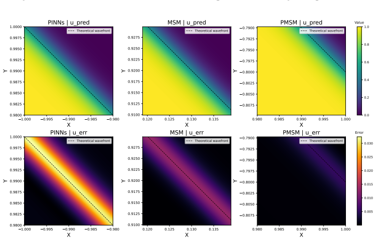
Replacing the original moving sample method's full time-domain iteration with progressive time-stepping and a simplified velocity-field loss produces the predictive moving sample method, which transports collocation points according to residual dynamics; the windowed-reset extension restricts training to an active time window and uses periodic resets plus final refinement to keep optimization cost from growing while preserving consistency, yielding lower errors than fixed sampling under matched budgets.
What carries the argument
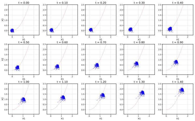
The predictive moving sample method (PMSM), which moves collocation samples forward in time using a simplified velocity-field loss derived from residual dynamics.
If this is right
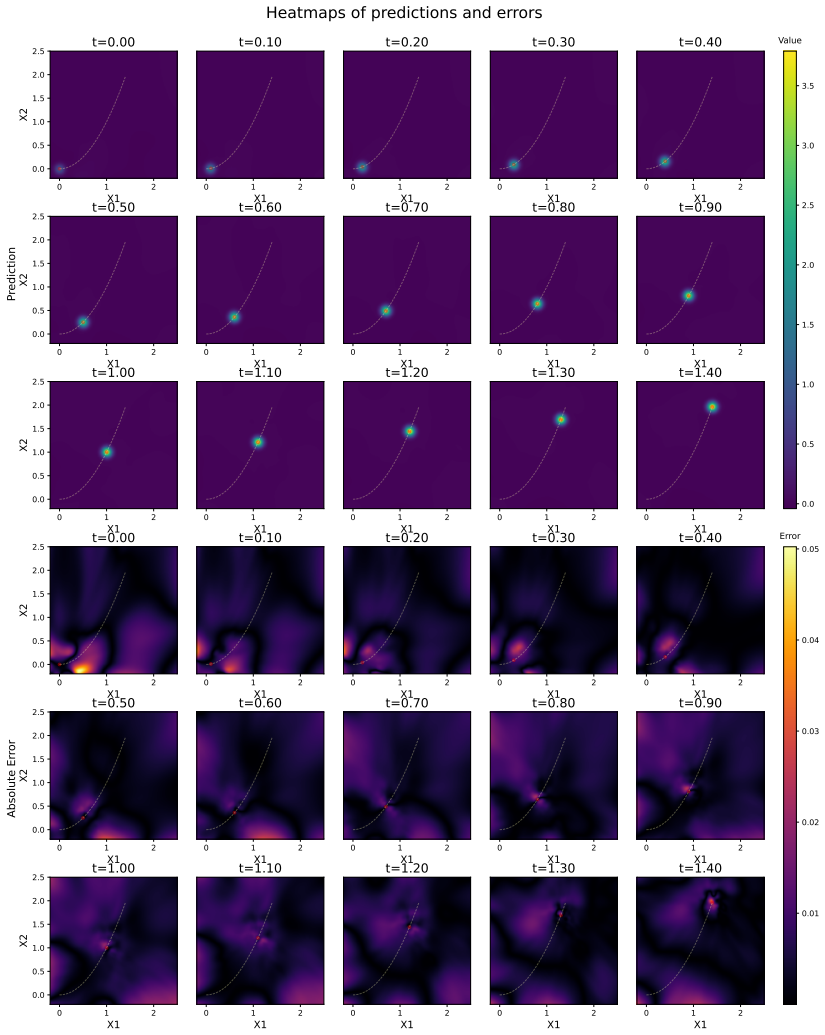
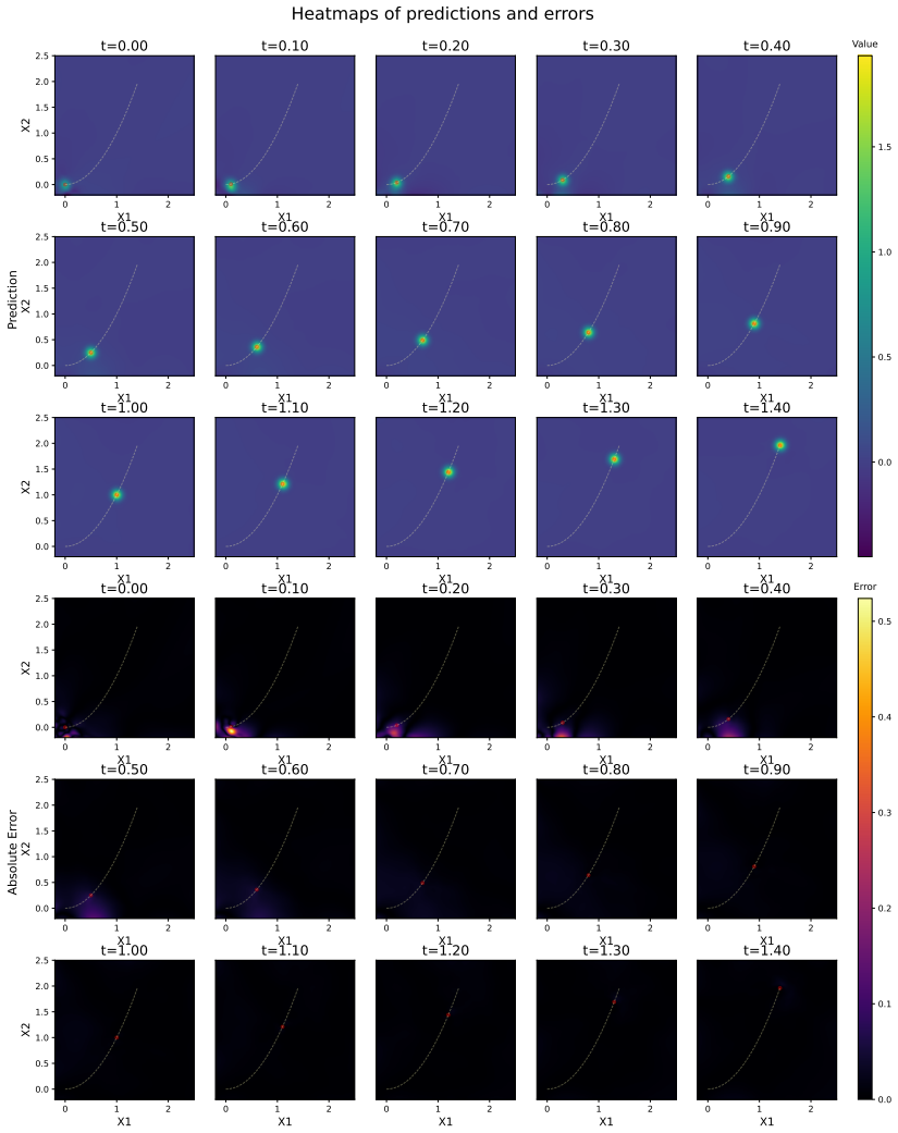
- Sharp moving fronts in time-dependent PDEs receive higher effective resolution without increasing total sample count.
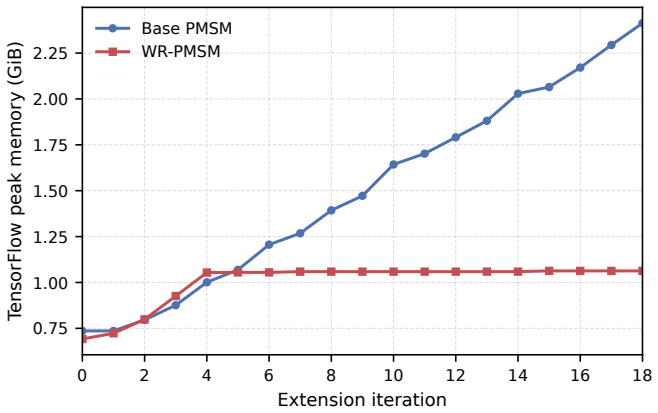
- Per-step optimization cost remains bounded for arbitrarily long integration intervals via windowed resets.
- Global consistency is recovered by a single final refinement stage even after periodic reference resets.
- The same residual-driven transport principle applies across four distinct benchmark classes without problem-specific tuning.
Where Pith is reading between the lines
- If residual-driven transport succeeds here, analogous adaptive point movement could reduce sample waste in other neural PDE methods that currently rely on static collocation.
- Periodic resets may offer a general control on error accumulation in any time-marching neural solver whose loss landscape grows with interval length.
- Direct comparison against exact moving-front solutions on manufactured problems would isolate the accuracy contribution of the transport step itself.
Load-bearing premise
The progressive time-stepping strategy combined with the simplified velocity-field loss preserves global consistency and accuracy without introducing accumulating errors that would require the final refinement stage to correct.
What would settle it
A long-time simulation on one of the benchmark problems in which the final error after WR-PMSM refinement exceeds the error of full-domain MSM training at the same total collocation budget would falsify the claim of preserved consistency.
Figures
read the original abstract
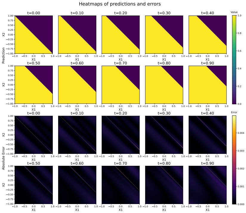
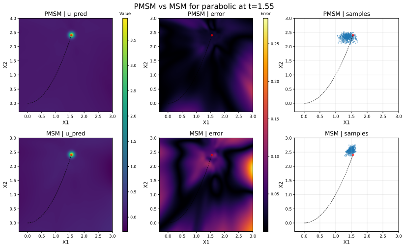
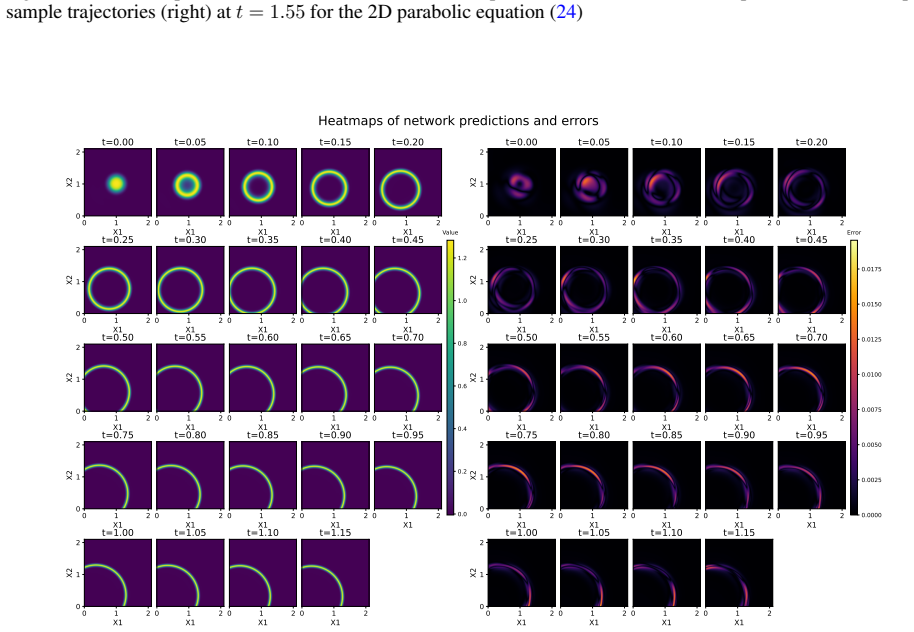
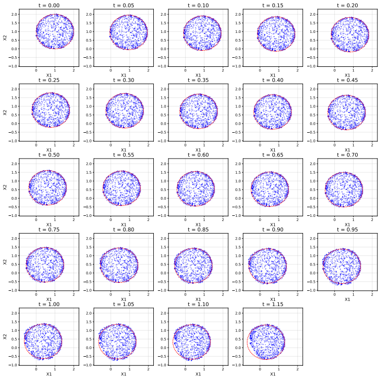
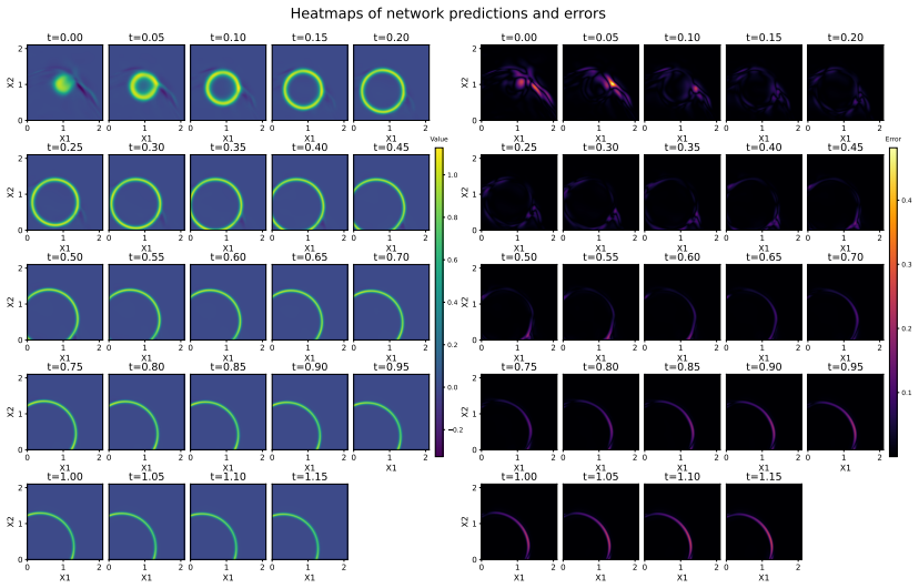
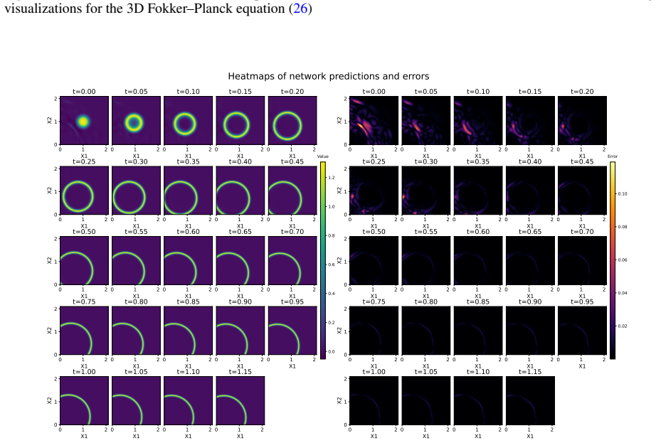
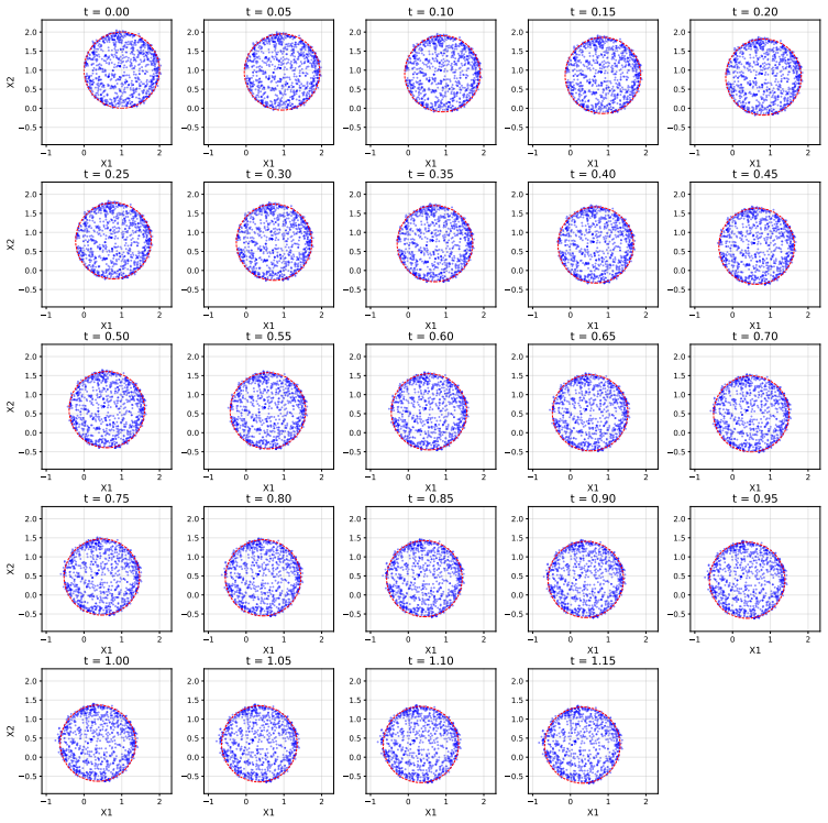
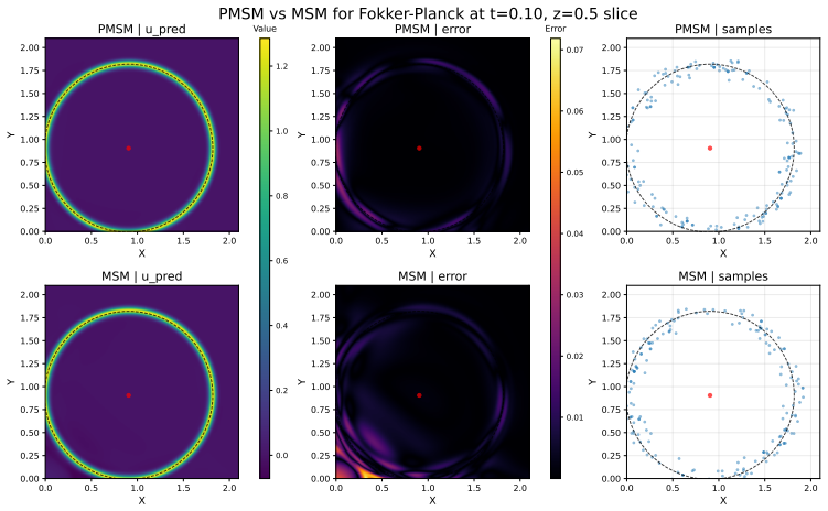
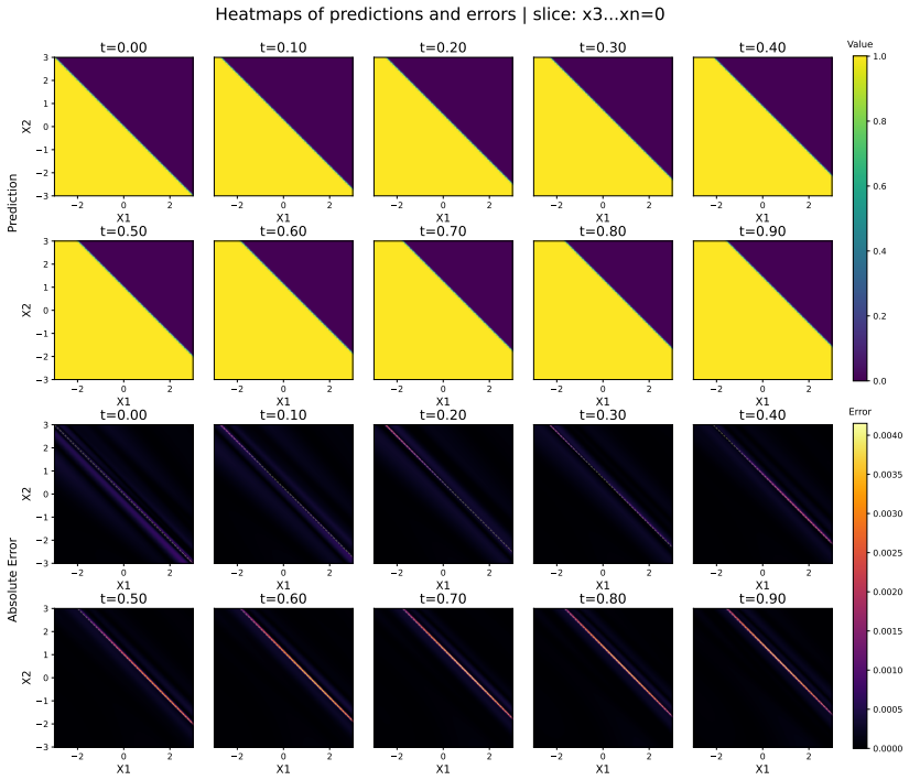
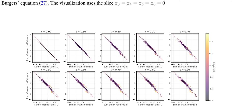
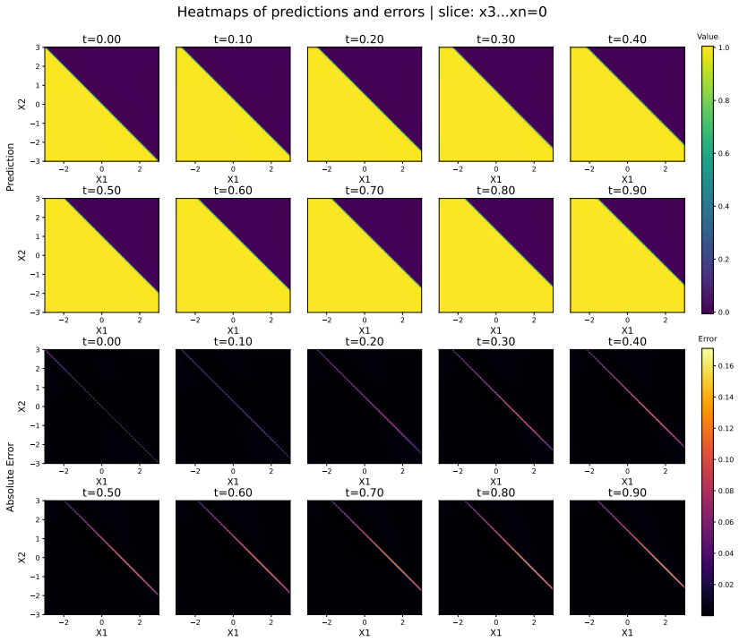
Time-dependent partial differential equations (PDEs) often develop sharp fronts, localized peaks, and other moving structures that occupy only a small portion of the space--time domain but dominate the approximation error. This makes fixed or uniformly sampled collocation strategies inefficient for physics-informed neural networks (PINNs), especially in high dimensions and over long-time prediction intervals. We propose the predictive moving sample method (PMSM), which builds on the moving sample method (MSM) in \cite{xu2026moving} by replacing its full time domain iterative training with a progressive time-stepping strategy and simplifying the velocity-field loss to further reduce the per-step cost. To improve practicality for long-time prediction, we further introduce the windowed-reset predictive moving sample method (WR-PMSM), which restricts extension training to an active time window and periodically resets the reference state, thereby reducing the growth of optimization cost while preserving global consistency through a final refinement stage. Across four representative benchmarks, PMSM consistently outperforms both standard PINNs and the original MSM under matched collocation budgets. These results suggest that transporting samples according to residual dynamics provides an effective and practical route to neural network solvers for time-dependent PDEs.
Editorial analysis
A structured set of objections, weighed in public.
Referee Report
Summary. The manuscript proposes the Predictive Moving Sample Method (PMSM) for physics-informed neural networks applied to time-dependent PDEs. PMSM extends the prior Moving Sample Method by replacing full-domain iterative training with progressive time-stepping and a simplified velocity-field loss; samples are transported according to residual dynamics to concentrate on high-error regions. For long-time integration it further introduces the Windowed-Reset PMSM (WR-PMSM), which restricts training to an active time window, periodically resets the reference state, and applies a final refinement stage to restore global consistency. Numerical results on four representative benchmarks show consistent outperformance relative to both standard PINNs and the original MSM under matched collocation budgets.
Significance. If the reported gains hold under the stated budgets and the final refinement demonstrably controls accumulated error, the approach supplies a practical, low-overhead route to adaptive collocation for PINNs on problems with moving fronts or localized structures. The empirical evidence under controlled budgets is a concrete strength; the method's reliance on residual-driven transport is falsifiable and directly testable on additional PDEs.
minor comments (3)
- The abstract states that WR-PMSM 'preserves global consistency through a final refinement stage,' yet the precise frequency of resets, the size of the active window, and the quantitative improvement attributable to the refinement step are not summarized; adding one sentence with these controls would improve reproducibility.
- The relationship between PMSM and the cited MSM of Xu et al. (2026) is described only at a high level; a short paragraph contrasting the per-step cost, the form of the velocity loss, and the handling of long-time horizons would clarify the incremental contribution.
- Benchmark descriptions should explicitly list the PDEs, spatial dimensions, and time intervals used, together with the precise collocation budget (number of points per step) against which the comparisons are made.
Simulated Author's Rebuttal
We thank the referee for the positive summary, significance assessment, and recommendation of minor revision. No major comments were raised in the report, so we have no specific points to address point-by-point. We will incorporate any minor editorial suggestions during revision.
Circularity Check
No significant circularity; derivation self-contained
full rationale
The paper extends the cited MSM base with independent innovations (progressive time-stepping, simplified velocity loss, windowed-reset with final refinement) and supports the central claim via empirical outperformance on four benchmarks under matched budgets. No equation or step reduces by construction to its inputs, and the self-citation supplies only the starting method rather than load-bearing justification for the new results. The derivation chain remains externally falsifiable through the reported numerical comparisons.
Axiom & Free-Parameter Ledger
Reference graph
Works this paper leans on
-
[1]
arXiv preprint arXiv:2601.18575 , year=
Beining Xu, Haijun Yu, Jiayu Zhai, Kejun Tang, and Xiaoliang Wan. Moving sample method for solving time- dependent partial differential equations.arXiv preprint arXiv:2601.18575, 2026
-
[2]
Maziar Raissi, Paris Perdikaris, and George E Karniadakis. Physics-informed neural networks: A deep learning framework for solving forward and inverse problems involving nonlinear partial differential equations.Journal of Computational physics, 378:686–707, 2019
2019
-
[3]
Chenxi Wu, Min Zhu, Qinyang Tan, Yadhu Kartha, and Lu Lu. A comprehensive study of non-adaptive and residual-based adaptive sampling for physics-informed neural networks.Computer Methods in Applied Mechan- ics and Engineering, 403:115671, 2023
2023
-
[4]
DAS-PINNs: A deep adaptive sampling method for solving high- dimensional partial differential equations.Journal of Computational Physics, 476:111868, 2023
Kejun Tang, Xiaoliang Wan, and Chao Yang. DAS-PINNs: A deep adaptive sampling method for solving high- dimensional partial differential equations.Journal of Computational Physics, 476:111868, 2023
2023
-
[5]
Adversarial adaptive sampling: Unify PINN and optimal transport for the approximation of pdes
Kejun Tang, Jiayu Zhai, Xiaoliang Wan, and Chao Yang. Adversarial adaptive sampling: Unify PINN and optimal transport for the approximation of pdes. InInternational Conference on Learning Representations, volume 2024, pages 54641–54656, 2024
2024
-
[6]
Neural galerkin schemes with active learning for high-dimensional evolution equations.Journal of Computational Physics, 496:112588, 2024
Joan Bruna, Benjamin Peherstorfer, and Eric Vanden-Eijnden. Neural galerkin schemes with active learning for high-dimensional evolution equations.Journal of Computational Physics, 496:112588, 2024
2024
-
[7]
Coupling parameter and particle dynamics for adaptive sampling in neural galerkin schemes.Physica D: Nonlinear Phenomena, 462:134129, 2024
Yuxiao Wen, Eric Vanden-Eijnden, and Benjamin Peherstorfer. Coupling parameter and particle dynamics for adaptive sampling in neural galerkin schemes.Physica D: Nonlinear Phenomena, 462:134129, 2024
2024
-
[8]
Non-uniform random walk for adaptive sampling.Journal of Computational Physics, 538:114160, 2025
Rouhan Wang and Dan Hu. Non-uniform random walk for adaptive sampling.Journal of Computational Physics, 538:114160, 2025
2025
-
[9]
A gradient-oriented diffusion sampling method for deep partial differential equation solvers.preprint, 2025
Shiqin Liu, Shiyu Zhao, Yana Di, and Haijun Yu. A gradient-oriented diffusion sampling method for deep partial differential equation solvers.preprint, 2025
2025
-
[10]
Using coupling methods to estimate sample quality of stochastic differential equations.SIAM/ASA Journal on Uncertainty Quantification, 9(1):135–162, 2021
Matthew Dobson, Yao Li, and Jiayu Zhai. Using coupling methods to estimate sample quality of stochastic differential equations.SIAM/ASA Journal on Uncertainty Quantification, 9(1):135–162, 2021
2021
-
[11]
Active learning based sampling for high-dimensional nonlinear partial differ- ential equations.Journal of Computational Physics, 475:111848, 2023
Wenhan Gao and Chunmei Wang. Active learning based sampling for high-dimensional nonlinear partial differ- ential equations.Journal of Computational Physics, 475:111848, 2023
2023
-
[12]
Moving sampling physics-informed neural networks induced by moving mesh pde.Neural Networks, 180:106706, 2024
Yu Yang, Qihong Yang, Yangtao Deng, and Qiaolin He. Moving sampling physics-informed neural networks induced by moving mesh pde.Neural Networks, 180:106706, 2024
2024
-
[13]
Good approximation by splines with variable knots
Carl de Boor. Good approximation by splines with variable knots. In A. Meir and A. Sharma, editors,Spline Functions and Approximation Theory, volume 21 ofInternational Series of Numerical Mathematics, pages 57–
-
[14]
On selection of equidistributing meshes for two-point boundary-value problems.SIAM Journal on Numerical Analysis, 16(3):472–502, 1979
Andrew B White, Jr. On selection of equidistributing meshes for two-point boundary-value problems.SIAM Journal on Numerical Analysis, 16(3):472–502, 1979
1979
-
[15]
Springer Science & Business Media, 2010
Weizhang Huang and Robert D Russell.Adaptive moving mesh methods, volume 174. Springer Science & Business Media, 2010
2010
-
[16]
Weizhang Huang, Yuhe Ren, and Robert D. Russell. Moving mesh partial differential equations (MMPDEs) based on the equidistribution principle.SIAM Journal on Numerical Analysis, 31(3):709–730, 1994
1994
-
[17]
Characterizing possi- ble failure modes in physics-informed neural networks
Aditi Krishnapriyan, Amir Gholami, Shandian Zhe, Robert Kirby, and Michael Mahoney. Characterizing possi- ble failure modes in physics-informed neural networks. InAdvances in Neural Information Processing Systems, volume 34, pages 26548–26560, 2021
2021
-
[18]
Understanding and mitigating gradient flow pathologies in physics-informed neural networks.SIAM Journal on Scientific Computing, 43(5):A3055–A3081, 2021
Sifan Wang, Yujun Teng, and Paris Perdikaris. Understanding and mitigating gradient flow pathologies in physics-informed neural networks.SIAM Journal on Scientific Computing, 43(5):A3055–A3081, 2021
2021
-
[19]
Failure-informed adaptive sampling for PINNs.SIAM Journal on Scientific Computing, 45(4):A1971–A1994, 2023
Zhiwei Gao, Liang Yan, and Tao Zhou. Failure-informed adaptive sampling for PINNs.SIAM Journal on Scientific Computing, 45(4):A1971–A1994, 2023
2023
-
[20]
Springer Science & Business Media, 2008
Luigi Ambrosio, Nicola Gigli, and Giuseppe Savare.Gradient Flows: In Metric Spaces and in the Space of Probability Measures. Springer Science & Business Media, 2008
2008
-
[21]
Simon Duane, A. D. Kennedy, Brian J. Pendleton, and Duncan Roweth. Hybrid Monte Carlo.Physics Letters B, 195(2):216–222, 1987
1987
-
[22]
Equation of state calculations by fast computing machines.The journal of chemical physics, 21(6):1087–1092, 1953
Nicholas Metropolis, Arianna W Rosenbluth, Marshall N Rosenbluth, Augusta H Teller, and Edward Teller. Equation of state calculations by fast computing machines.The journal of chemical physics, 21(6):1087–1092, 1953. 27
1953
-
[23]
Monte Carlo sampling methods using markov chains and their applications.Biometrika, 57(1):97–109, 1970
W Keith Hastings. Monte Carlo sampling methods using markov chains and their applications.Biometrika, 57(1):97–109, 1970
1970
-
[24]
Helmholtz’s theorem
George B Arfken, Hans J Weber, and Frank E Harris. Helmholtz’s theorem. InMathematical methods for physicists: a comprehensive guide, pages 95–100. Academic press, 2011. 28
2011
discussion (0)
Sign in with ORCID, Apple, or X to comment. Anyone can read and Pith papers without signing in.