MATLAB-Based Layerwise Self-Adaptive Physics-Informed Neural Network in Applications to Multidimensional Coupled Burgers' Equations with High Reynolds Numbers
Pith reviewed 2026-06-27 08:54 UTC · model grok-4.3
The pith
A layerwise self-adaptive weighting strategy in PINNs improves accuracy and shock capture for multidimensional coupled Burgers' equations at high Reynolds numbers.
A machine-rendered reading of the paper's core claim, the machinery that carries it, and where it could break.
Core claim
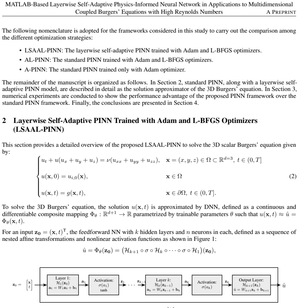
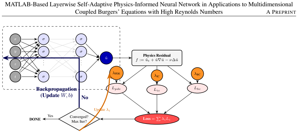
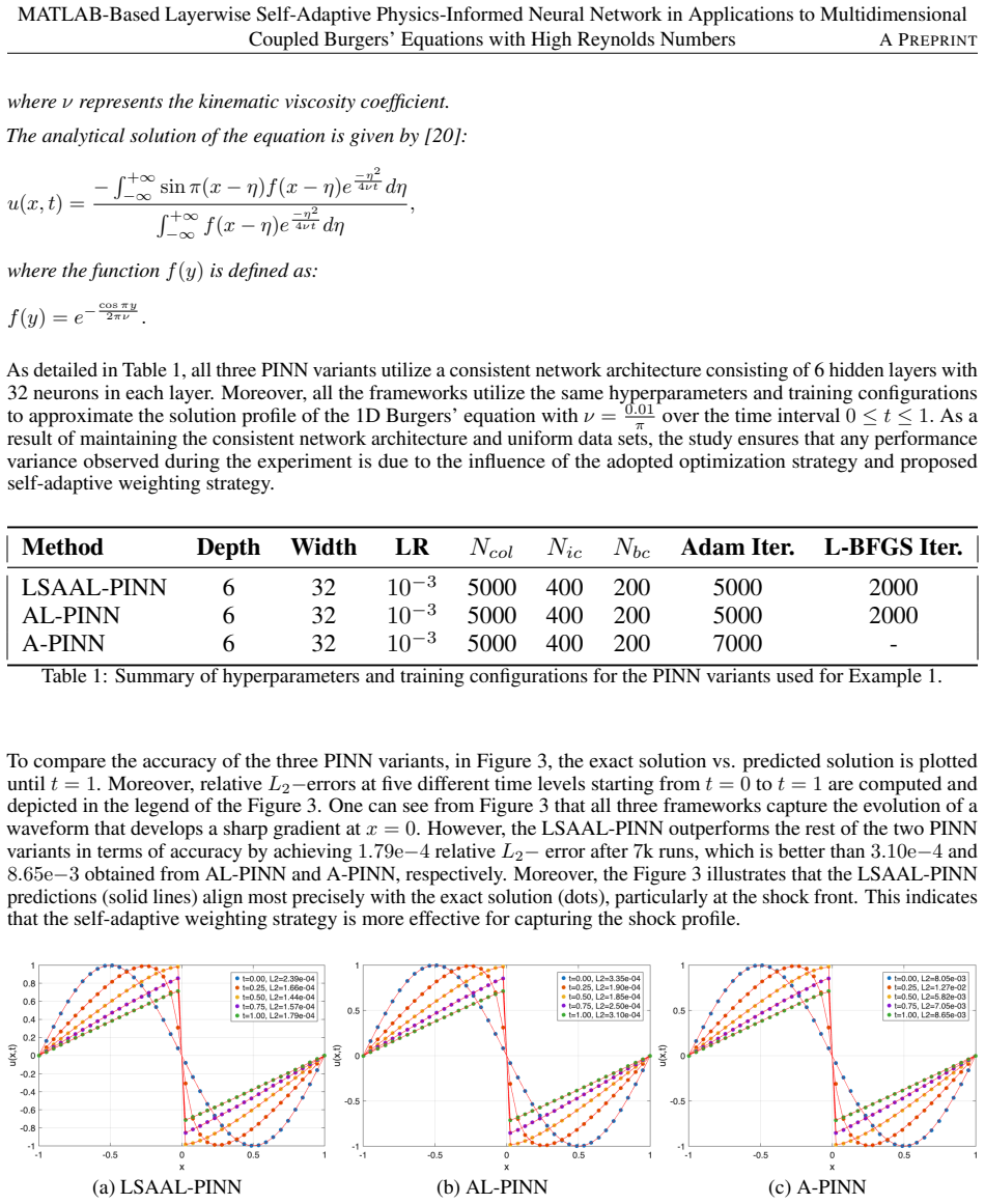
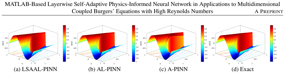
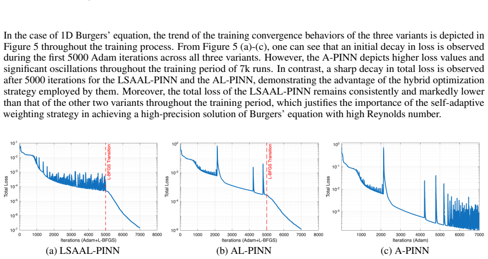
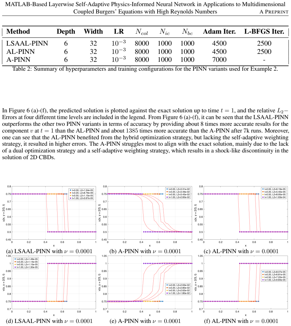
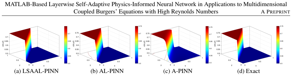
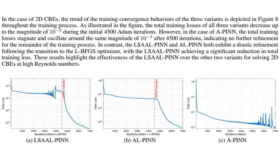
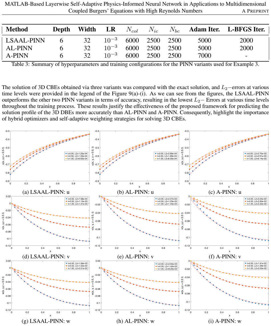
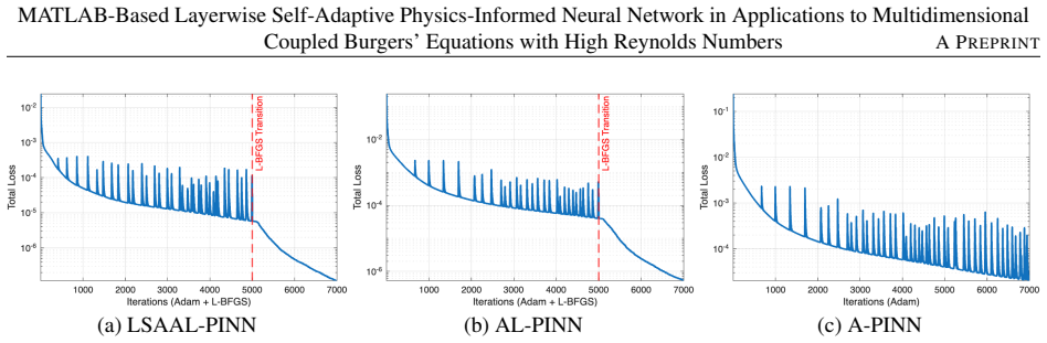
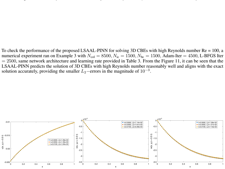
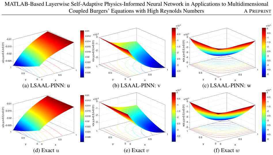
The proposed framework employs a layerwise self-adaptive weighting strategy that dynamically adjusts the penalty weights for the physics residual, initial conditions, and boundary conditions throughout training. Moreover, the framework uses a dual-phase optimization strategy to achieve more stable convergence. Numerical results exhibit that the proposed framework achieves higher accuracy in terms of relative L2-error norm than the standard PINN and is able to capture the development of sharp shock fronts as time evolves in the solution.
What carries the argument
The layerwise self-adaptive weighting strategy that dynamically adjusts penalty weights for physics residual, initial conditions, and boundary conditions, together with dual-phase optimization.
If this is right
- Higher relative L2-error accuracy than standard PINN with or without L-BFGS optimization.
- Successful tracking of sharp shock fronts that develop over time.
- More stable convergence during training on the target equations.
- Applicability to both one- and multi-dimensional versions of the coupled system.
Where Pith is reading between the lines
- The same weighting mechanism could be tested on other nonlinear hyperbolic or convection-dominated PDEs that develop discontinuities.
- Because the implementation is in MATLAB, it may lower the barrier for engineers already using that environment to try physics-informed networks.
- The dual-phase schedule might interact with network depth or activation choice in ways that warrant separate ablation on larger problems.
Load-bearing premise
The layerwise self-adaptive weighting and dual-phase optimization produce stable, generalizable accuracy gains and shock capture for high-Re cases without requiring problem-specific retuning or introducing new instabilities.
What would settle it
A test run on a fresh high-Reynolds-number multidimensional coupled Burgers' problem in which the proposed method yields equal or larger relative L2 error than a standard PINN or visibly fails to resolve the emerging shock fronts.
Figures
read the original abstract
This paper presents an improved physics-informed neural network for simulating the spatio-temporal solution profile of the multidimensional coupled Burgers' equations with high Reynolds numbers. As time evolves, the sharp shock fronts emerge in the solution, creating significant computational challenges for the conventional mesh-based numerical methods. In particular, numerical methods such as finite differences and finite elements suffer from poor stability and strong mesh dependency when resolving the steep solution gradients. To address these challenges, the proposed framework employs a layerwise self-adaptive weighting strategy that dynamically adjusts the penalty weights for the physics residual, initial conditions, and boundary conditions throughout training. Moreover, the framework uses a dual-phase optimization strategy to achieve more stable convergence. To check the effectiveness and accuracy of the proposed framework, a set of numerical experiments is conducted to compare it with the standard Physics-Informed Neural Network (PINN) with and without Limited-memory Broyden-Fletcher-Goldfarb-Shanno (L-BFGS) optimization. Numerical results exhibit that the proposed framework achieves higher accuracy in terms of relative $L_2-$ error norm than the standard PINN and is able to capture the development of sharp shock fronts as time evolves in the solution.
Editorial analysis
A structured set of objections, weighed in public.
Referee Report
Summary. The paper proposes a MATLAB-based layerwise self-adaptive physics-informed neural network (PINN) with dual-phase optimization for multidimensional coupled Burgers' equations at high Reynolds numbers. It employs dynamic adjustment of penalty weights for physics residuals, initial conditions, and boundary conditions, claiming superior relative L2 accuracy and improved capture of sharp shock fronts compared to standard PINN (with and without L-BFGS).
Significance. If the numerical improvements hold under scrutiny, the layerwise self-adaptive weighting and dual-phase strategy could offer a practical enhancement for training stability in PINNs applied to convection-dominated PDEs with steep gradients, where mesh-based methods often fail.
major comments (1)
- [Abstract] Abstract: the central claim that 'numerical results exhibit that the proposed framework achieves higher accuracy in terms of relative L2-error norm' is presented without any specific error values, tables, baseline comparisons, network sizes, or training details, which is load-bearing for assessing whether the method actually outperforms standard PINN.
minor comments (2)
- [Abstract] The abstract introduces 'layerwise self-adaptive weighting strategy' and 'dual-phase optimization strategy' without equations or pseudocode, making it hard to understand the precise implementation even at a high level.
- [Abstract] No mention of the specific form of the multidimensional coupled Burgers' equations (e.g., the exact system solved) or the range of Reynolds numbers tested.
Simulated Author's Rebuttal
We thank the referee for their detailed review and constructive feedback. We address the major comment below and agree that revisions to the abstract are warranted to better support our claims with quantitative details from the full manuscript.
read point-by-point responses
-
Referee: [Abstract] Abstract: the central claim that 'numerical results exhibit that the proposed framework achieves higher accuracy in terms of relative L2-error norm' is presented without any specific error values, tables, baseline comparisons, network sizes, or training details, which is load-bearing for assessing whether the method actually outperforms standard PINN.
Authors: We agree that the abstract would be strengthened by including specific quantitative results. The full manuscript contains detailed comparisons in the numerical experiments section, including tables of relative L2 errors for the proposed method versus standard PINN (with and without L-BFGS), along with network architectures, training details, and Reynolds number cases. To address this point, we will revise the abstract to incorporate key error values and baseline comparisons from those experiments, ensuring the central claim is supported by specifics. revision: yes
Circularity Check
No significant circularity
full rationale
The paper describes an empirical method (layerwise self-adaptive weighting plus dual-phase optimization) for PINNs applied to high-Re Burgers' equations and validates it via direct numerical comparisons of relative L2 error against standard PINN on the same test problems. No derivation chain exists that reduces a claimed result to its own fitted parameters or to a self-citation; the reported improvements are external benchmarks, not quantities defined in terms of the method itself.
Axiom & Free-Parameter Ledger
Reference graph
Works this paper leans on
-
[1]
Sanchez-Lengeling, A
B. Sanchez-Lengeling, A. Aspuru-Guzik, A gentle introduction to deep learning in molecules, Science 361 (2018) 360-365
2018
-
[2]
Hinton, L
G. Hinton, L. Deng, D. Yu, G. E. Dahl, A-r. Mohamed, N. Jaitly, A. Senior, V . Vanhoucke, P. Nguyen, T. N. Sainath, B. Kingsbury, Deep neural networks for acoustic modeling in speech recognition: The shared views of four research groups, IEEE Signal Process. Mag. 29 (2012) 82-97
2012
-
[3]
Krizhevsky, I
A. Krizhevsky, I. Sutskever, G. Hinton, ImageNet classification with deep convolutional neural networks, Adv. Neural Inf. Process. Syst. 25 (2012), 1097–1105
2012
-
[4]
J. Pathak, S. Subramanian, P. Harrington, S. Raja, A. Chattopadhyay, M. Mardani, T. Kurth, D. Hall, Z. Li, K. Azizzadenesheli, et al., FourCastNet: A global data-driven high-resolution weather model using adaptive Fourier neural operators, arXiv preprint arXiv:2202.11214 (2022)
work page internal anchor Pith review Pith/arXiv arXiv 2022
-
[5]
Y . Wu, M. Schuster, Z. Chen, Q. V . Le, M. Norouzi, W. Macherey, M. Krikun, Y . Cao, Q. Gao, K. Macherey, et al., Google’s neural machine translation system: Bridging the gap between human and machine translation, arXiv preprint arXiv:1609.08144 (2016)
work page internal anchor Pith review Pith/arXiv arXiv 2016
-
[6]
Jumper, R
J. Jumper, R. Evans, B. Pritzel, T. Green, M. Figurnov, O. Ronneberger, K. Tunyasuvunakool, R. Bates, A. Žídek, A. Potapenko, et al., Highly accurate protein structure prediction with AlphaFold, Nature 596 (2021) 583-589
2021
-
[7]
Raissi, P
M. Raissi, P. Perdikaris, G. E. Karniadakis, Physics-informed neural networks: A deep learning framework for solving forward and inverse problems involving nonlinear partial differential equations, J. Comput. Phys. 378 (2019) 686-707. 12 MATLAB-Based Layerwise Self-Adaptive Physics-Informed Neural Network in Applications to Multidimensional Coupled Burger...
2019
-
[8]
Di Bella, D
A. Di Bella, D. Santoro, M. Raissi, P. Roccaro, Physics-informed neural networks in water and wastewater systems: a critical review. Water Res. 288 (2026), 125449
2026
-
[9]
Quarteroni, A
A. Quarteroni, A. Valli, Numerical approximation of partial differential equations, Springer Science & Business Media, (2008)
2008
-
[10]
A. D. Jagtap, E. Kharazmi, G. E. Karniadakis, Conservative physics-informed neural networks on discrete domains for conservation laws: Applications to forward and inverse problems, Comput. Methods Appl. Mech. Eng. 365 (2020), 113028
2020
-
[11]
X. Meng, Z. Li, D. Zhang, G. E. Karniadakis, PPINN: Parareal physics-informed neural network for time- dependent PDEs, Comput. Methods Appl. Mech. Eng. 370 (2020), 113250
2020
-
[12]
Mattey, S
R. Mattey, S. Ghosh, A novel sequential method to train physics informed neural networks for Allen Cahn and Cahn Hilliard equations, Comput. Methods Appl. Mech. Eng. 390 (2022), 114474
2022
-
[13]
L. D. McClenny, U. M. Braga-Neto, Self-adaptive physics-informed neural networks. J. Comput. Phys. 474 (2023), 111722
2023
-
[14]
R. D. Ortiz Ortiz, O. Martínez Núñez, A. M. Marín Ramírez, Solving Viscous Burgers’ Equation: Hybrid Approach Combining Boundary Layer Theory and Physics-Informed Neural Networks. Mathematics 12 (2024), 3430
2024
-
[15]
Y . Song, H. Wang, H. Yang, M. L. Taccari, X. Chen, Loss-attentional physics-informed neural networks, J. Comput. Phys. 501 (2024), 112781
2024
-
[16]
X. Wang, S. Yi, H. Gu, J. Xu, W. Xu, WF-PINNs: solving forward and inverse problems of the Burgers equation with steep gradients using weak-form physics-informed neural networks, Sci. Rep. 15(1) (2025), 40555
2025
-
[17]
Zhang, C
Z. Zhang, C. Ruan, Z. Liu, Two improved physics-informed Neural Networks for solving Burgers equation. J. Comput. Sci. 93 (2026), 102756
2026
-
[18]
Glorot, Y
X. Glorot, Y . Bengio, Understanding the difficulty of training deep feedforward neural networks, in: Proceedings of the thirteenth international conference on artificial intelligence and statistics, JMLR Workshop and Conference Proceedings (2010), 249–256
2010
-
[19]
Stein, Large sample properties of simulations using Latin hypercube sampling, Technometrics 29 (1987), 143–151
M. Stein, Large sample properties of simulations using Latin hypercube sampling, Technometrics 29 (1987), 143–151
1987
-
[20]
Basdevant, M
C. Basdevant, M. Deville, P. Haldenwang, J.M. Lacroix, J. Ouazzani, R. Peyret, P. Orlandi, and A.T. Patera, Spectral and finite difference solutions of the Burgers equation, Comput. Fluids 14 (1986), 23-41
1986
-
[21]
C. A. J. Fletcher, Generating exact solutions of the two-dimensional Burgers’ equations, Int. J. Numer. Methods Fluids 3 (1983) 213-216
1983
-
[22]
H. S. Shukla, M. Tamsir, V . K. Srivastava, and M. M. Rashidi, Modified cubicβ-spline differential quadrature method for numerical solution of three-dimensional coupled viscous Burger equation, Mod. Phys. Lett. B 30 (2016), 1650110. 13
2016
discussion (0)
Sign in with ORCID, Apple, or X to comment. Anyone can read and Pith papers without signing in.