Establishing an Ω(sqrt{d}) complexity lower bound for PDMP samplers and how to break it: a sub-sqrt{d} algorithm for Gaussian-tailed targets
Pith reviewed 2026-06-26 15:18 UTC · model grok-4.3
The pith
Standard PDMP samplers face an Ω(√d) complexity lower bound, but a new scheme that relaxes continuous invariance achieves O(d^α) scaling with α in [0.2, 0.3] for Gaussian-tailed targets.
A machine-rendered reading of the paper's core claim, the machinery that carries it, and where it could break.
Core claim
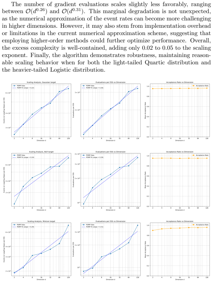
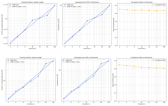
We prove that this is a fundamental limitation by establishing an Ω(√d) lower bound on the algorithmic complexity of PDMP samplers in a standard setup. By relaxing the assumption that the target density must remain invariant at all continuous times, we then demonstrate how to bypass this barrier. Specifically, we introduce a novel PDMP sampling scheme and show that it achieves an empirical complexity of O(d^α), where α ∈ [0.2, 0.3] for Gaussian-tailed targets. In addition, this PDMP scheme is locally adaptive in both trajectory length and distance between velocity updates.
What carries the argument
A novel PDMP sampling scheme that relaxes continuous-time target invariance while adapting locally to trajectory length and inter-update distances.
If this is right
- Standard PDMP samplers cannot scale better than Ω(√d) under the continuous-invariance requirement.
- The new scheme achieves empirical O(d^α) complexity with α ∈ [0.2, 0.3] on Gaussian-tailed targets.
- The scheme adapts locally to both trajectory length and distance between velocity updates.
- Relaxing continuous invariance is sufficient to bypass the proven lower bound.
Where Pith is reading between the lines
- The same relaxation of invariance might be tested on other families of non-reversible samplers to check whether comparable dimension gains appear.
- If the local adaptation rules generalize, the method could be tried on targets whose tails decay faster or slower than Gaussian.
- In applied settings the reduced exponent would directly lower the dimension at which posterior sampling becomes practical for models with roughly Gaussian posteriors.
Load-bearing premise
The lower bound requires that the target density remain invariant at every continuous time.
What would settle it
A concrete counter-example would be any PDMP sampler that achieves better than √d scaling while keeping the target density invariant at all continuous times; for the new scheme, failure to observe O(d^α) with α < 0.5 on standard Gaussian-tailed test problems would challenge the bypass.
Figures
read the original abstract
Despite the theoretical appeal of their non-reversibility, to date, no Piecewise Deterministic Markov Process (PDMP) samplers have been developed that scale better than $\mathcal{O}(\sqrt{d})$ in computational complexity with respect to the target dimension $d$. We prove that this is a fundamental limitation by establishing an $\Omega(\sqrt{d})$ lower bound on the algorithmic complexity of PDMP samplers in a standard setup. By relaxing the assumption that the target density must remain invariant at all continuous times, we then demonstrate how to bypass this barrier. Specifically, we introduce a novel PDMP sampling scheme and show that it achieves an empirical complexity of $\mathcal{O}(d^\alpha)$, where $\alpha \in [0.2, 0.3]$ for Gaussian-tailed targets. In addition, this PDMP scheme is locally adaptive in both trajectory length and distance between velocity updates.
Editorial analysis
A structured set of objections, weighed in public.
Referee Report
Summary. The paper proves an Ω(√d) lower bound on the algorithmic complexity of PDMP samplers under the standard setup requiring continuous-time invariance of the target density. It then introduces a novel PDMP scheme that relaxes this invariance, is locally adaptive in trajectory length and velocity-update distance, and empirically achieves O(d^α) complexity with α ∈ [0.2, 0.3] for Gaussian-tailed targets.
Significance. If the lower-bound proof is rigorous and the empirical complexity is counted on identical footing (same units of gradient/velocity-update cost per effective sample), the work would be significant: it both identifies a fundamental limit for invariant PDMPs and demonstrates a concrete way to circumvent it. The combination of a matching lower bound with a bypassing algorithm, plus the local adaptivity, strengthens the contribution.
major comments (3)
- [§3] §3 (lower-bound statement and proof): the definition of algorithmic complexity (velocity updates or gradient calls per effective sample) must be stated explicitly and shown to be identical to the metric used for the empirical scaling in §5; without this, the claim that the new scheme breaks the Ω(√d) bound cannot be verified.
- [§4.2] §4.2 (definition of the new scheme): the precise manner in which continuous-time invariance is relaxed is load-bearing for the bypass argument; the text must clarify whether the process remains a PDMP at every instant or only at discrete update times, and whether any additional overhead from the adaptation mechanism is charged to the complexity count.
- [§5] §5 (empirical complexity plots and tables): the reported α ∈ [0.2, 0.3] is obtained over which range of dimensions, and how is effective sample size computed (e.g., integrated autocorrelation time)? If the adaptation cost or trajectory-length overhead is omitted from the count, the apparent sub-√d scaling does not directly contradict the lower bound.
minor comments (2)
- [Abstract] Abstract: the phrase 'standard setup' should be defined in one sentence so readers immediately understand the invariance assumption being relaxed.
- [§2] Notation: the symbol for effective sample size or the precise complexity unit should be introduced once in §2 and used consistently thereafter.
Simulated Author's Rebuttal
We thank the referee for the careful reading and constructive comments. We address each major comment below and indicate the revisions that will be made.
read point-by-point responses
-
Referee: [§3] §3 (lower-bound statement and proof): the definition of algorithmic complexity (velocity updates or gradient calls per effective sample) must be stated explicitly and shown to be identical to the metric used for the empirical scaling in §5; without this, the claim that the new scheme breaks the Ω(√d) bound cannot be verified.
Authors: We agree that an explicit definition is required for the lower-bound claim to be verifiable. In the revised manuscript we will add a dedicated paragraph in §3 that defines algorithmic complexity precisely as the number of velocity updates plus gradient evaluations per effective sample, and we will insert a sentence confirming that the identical metric is used for the empirical scaling reported in §5. revision: yes
-
Referee: [§4.2] §4.2 (definition of the new scheme): the precise manner in which continuous-time invariance is relaxed is load-bearing for the bypass argument; the text must clarify whether the process remains a PDMP at every instant or only at discrete update times, and whether any additional overhead from the adaptation mechanism is charged to the complexity count.
Authors: The scheme preserves the PDMP structure on each inter-update interval while relaxing continuous-time invariance of the target density so that invariance holds only at the discrete update instants. All costs incurred by the local adaptation rules (trajectory-length selection and velocity-update distances) are included in the complexity count. We will revise §4.2 to state these facts explicitly. revision: yes
-
Referee: [§5] §5 (empirical complexity plots and tables): the reported α ∈ [0.2, 0.3] is obtained over which range of dimensions, and how is effective sample size computed (e.g., integrated autocorrelation time)? If the adaptation cost or trajectory-length overhead is omitted from the count, the apparent sub-√d scaling does not directly contradict the lower bound.
Authors: We will add to §5 the exact range of dimensions over which the reported scaling was observed, confirm that effective sample size is obtained from the integrated autocorrelation time, and state that every adaptation and trajectory-length cost is charged to the complexity metric. These additions will make the empirical results directly comparable to the lower bound. revision: yes
Circularity Check
No significant circularity; lower bound and empirical bypass are independent.
full rationale
The paper states an Ω(√d) lower bound for PDMPs under the standard invariance-at-all-times assumption, then relaxes that assumption to introduce a new scheme with reported O(d^α) empirical scaling (α ∈ [0.2,0.3]). No equations, definitions, or self-citations are shown that reduce the lower bound or the complexity metric to a fitted quantity or prior result by construction. The central claims remain self-contained against external benchmarks; the relaxation explicitly addresses the bound's premise rather than redefining it.
Axiom & Free-Parameter Ledger
Reference graph
Works this paper leans on
-
[1]
Charly Andral and Kengo Kamatani. Automated techniques for effi- cient sampling of piecewise-deterministic Markov processes.arXiv preprint arXiv:2408.03682, 2024. 24
arXiv 2024
-
[2]
Optimal tuning of the hybrid Monte Carlo algorithm.Bernoulli, 19(5A):1501–1534, 2013
Alexandros Beskos, Natesh Pillai, Gareth Roberts, Jesus-Maria Sanz- Serna, and Andrew Stuart. Optimal tuning of the hybrid Monte Carlo algorithm.Bernoulli, 19(5A):1501–1534, 2013
2013
-
[3]
A conceptual introduction to Hamiltonian Monte Carlo.arXiv preprint arXiv:1701.02434, 2017
Michael Betancourt. A conceptual introduction to Hamiltonian Monte Carlo.arXiv preprint arXiv:1701.02434, 2017
Pith/arXiv arXiv 2017
-
[4]
The zig-zag process and super-efficient sampling for Bayesian analysis of big data
Joris Bierkens, Paul Fearnhead, and Gareth Roberts. The zig-zag process and super-efficient sampling for Bayesian analysis of big data. 2019
2019
-
[5]
The boomerang sampler
Joris Bierkens, Sebastiano Grazzi, Kengo Kamatani, and Gareth Roberts. The boomerang sampler. InInternational conference on machine learning, pages 908–918. PMLR, 2020
2020
-
[6]
The within-orbit adaptive leapfrog no-u-turn sampler.arXiv preprint arXiv:2506.18746, 2025
Nawaf Bou-Rabee, Bob Carpenter, Tore Selland Kleppe, and Sifan Liu. The within-orbit adaptive leapfrog no-u-turn sampler.arXiv preprint arXiv:2506.18746, 2025
arXiv 2025
-
[7]
Incorporating local step-size adaptivity into the no-u-turn sampler using gibbs self-tuning.The Journal of Chemical Physics, 163(8):084119, 08 2025
Nawaf Bou-Rabee, Bob Carpenter, Tore Selland Kleppe, and Milo Marsden. Incorporating local step-size adaptivity into the no-u-turn sampler using gibbs self-tuning.The Journal of Chemical Physics, 163(8):084119, 08 2025
2025
-
[8]
Nawaf Bou-Rabee, Bob Carpenter, and Milo Marsden. Gist: Gibbs self-tuning for locally adaptive hamiltonian monte carlo.arXiv preprint arXiv:2404.15253, 2025
Pith/arXiv arXiv 2025
-
[9]
The bouncy particle sampler: A nonreversible rejection-free Markov chain Monte Carlo method.Journal of the American Statistical Association, 113(522):855–867, 2018
Alexandre Bouchard-Cˆ ot´ e, Sebastian J Vollmer, and Arnaud Doucet. The bouncy particle sampler: A nonreversible rejection-free Markov chain Monte Carlo method.Journal of the American Statistical Association, 113(522):855–867, 2018
2018
-
[10]
Towards practical pdmp sampling: Metropolis adjustments, locally adaptive step-sizes, and nuts-based time lengths, 2025
Augustin Chevallier, Sam Power, and Matthew Sutton. Towards practical pdmp sampling: Metropolis adjustments, locally adaptive step-sizes, and nuts-based time lengths, 2025
2025
-
[11]
Automatic zig-zag sampling in practice.Statistics and Computing, 32(6):107, 2022
Alice Corbella, Simon EF Spencer, and Gareth O Roberts. Automatic zig-zag sampling in practice.Statistics and Computing, 32(6):107, 2022
2022
-
[12]
Mark H. A. Davis.Markov Models and Optimization, volume 49 ofMono- graphs on Statistics and Applied Probability. Chapman & Hall, London, 1993
1993
-
[13]
Randomized Hamiltonian Monte Carlo as scaling limit of the bouncy particle sampler and dimension-free convergence rates.The Annals of Applied Probability, 31(6):2612 – 2662, 2021
George Deligiannidis, Daniel Paulin, Alexandre Bouchard-Cˆ ot´ e, and Ar- naud Doucet. Randomized Hamiltonian Monte Carlo as scaling limit of the bouncy particle sampler and dimension-free convergence rates.The Annals of Applied Probability, 31(6):2612 – 2662, 2021
2021
-
[14]
Piecewise deterministic Markov processes for continuous-time Monte Carlo
Paul Fearnhead, Joris Bierkens, Murray Pollock, and Gareth O Roberts. Piecewise deterministic Markov processes for continuous-time Monte Carlo. Statistical Science, 33(3):386–412, 2018. 25
2018
-
[15]
The no-u-turn sampler: adap- tively setting path lengths in Hamiltonian Monte Carlo.J
Matthew D Hoffman, Andrew Gelman, et al. The no-u-turn sampler: adap- tively setting path lengths in Hamiltonian Monte Carlo.J. Mach. Learn. Res., 15(1):1593–1623, 2014
2014
-
[16]
Liptser and Albert N
Robert S. Liptser and Albert N. Shiryaev.Theory of Martingales, vol- ume 49. Springer, 1989
1989
-
[17]
On time reversal of piecewise deterministic Markov processes.Electronic Journal of Probability, 18(1):1 – 29, 2013
Andreas L¨ opker and Zbigniew Palmowski. On time reversal of piecewise deterministic Markov processes.Electronic Journal of Probability, 18(1):1 – 29, 2013
2013
-
[18]
Martin, Oriol Abril-Pla, Jordan Deklerk, Seth D
Osvaldo A. Martin, Oriol Abril-Pla, Jordan Deklerk, Seth D. Axen, Colin Carroll, Ari Hartikainen, and Aki Vehtari. Arviz: a modular and flexible library for exploratory analysis of bayesian models.Journal of Open Source Software, 11(119):9889, 2026
2026
-
[19]
Chirag Modi. ATLAS: Adapting Trajectory Lengths and Step-Size for Hamiltonian Monte Carlo.arXiv preprint arXiv:2410.21587, 2024
arXiv 2024
-
[20]
Delayed rejection Hamilto- nian Monte Carlo for sampling multiscale distributions.Bayesian Analysis, 19(3):815 – 842, 2024
Chirag Modi, Alex Barnett, and Bob Carpenter. Delayed rejection Hamilto- nian Monte Carlo for sampling multiscale distributions.Bayesian Analysis, 19(3):815 – 842, 2024
2024
-
[21]
MCMC using Hamiltonian dynamics.Handbook of markov chain monte carlo, 2(11):2, 2011
Radford M Neal et al. MCMC using Hamiltonian dynamics.Handbook of markov chain monte carlo, 2(11):2, 2011
2011
-
[22]
Weak convergence and optimal scaling of random walk Metropolis algorithms.The annals of applied probability, 7(1):110–120, 1997
Gareth O Roberts, Andrew Gelman, and Walter R Gilks. Weak convergence and optimal scaling of random walk Metropolis algorithms.The annals of applied probability, 7(1):110–120, 1997
1997
-
[23]
Optimal scaling of discrete approximations to Langevin diffusions.Journal of the Royal Statistical Society: Series B (Statistical Methodology), 60(1):255–268, 1998
Gareth O Roberts and Jeffrey S Rosenthal. Optimal scaling of discrete approximations to Langevin diffusions.Journal of the Royal Statistical Society: Series B (Statistical Methodology), 60(1):255–268, 1998
1998
-
[24]
Concave-convex PDMP-based sam- pling.Journal of Computational and Graphical Statistics, 32(4):1425–1435, 2023
Matthew Sutton and Paul Fearnhead. Concave-convex PDMP-based sam- pling.Journal of Computational and Graphical Statistics, 32(4):1425–1435, 2023
2023
-
[25]
Sampling from multi- scale densities with delayed rejection generalized Hamiltonian Monte Carlo
Gilad Turok, Chirag Modi, and Bob Carpenter. Sampling from multi- scale densities with delayed rejection generalized Hamiltonian Monte Carlo. arXiv preprint arXiv:2406.02741, 2024. A Deferred Proofs A.1 Complexity lower bound A.2 Detailed proof of Proposition 1 We start by two useful lemmas before the proof of the proposition itself. 26 Lemma 2(Lower Boun...
arXiv 2024
discussion (0)
Sign in with ORCID, Apple, or X to comment. Anyone can read and Pith papers without signing in.