When Entropy flows: drifting along the route to Chaos
Pith reviewed 2026-06-25 22:08 UTC · model grok-4.3
The pith
The Entropy flow extends any one-parameter family of vector fields with a parameter drift that drives trajectories from order to chaos.
A machine-rendered reading of the paper's core claim, the machinery that carries it, and where it could break.
Core claim
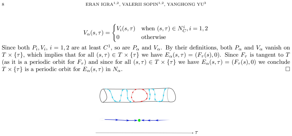
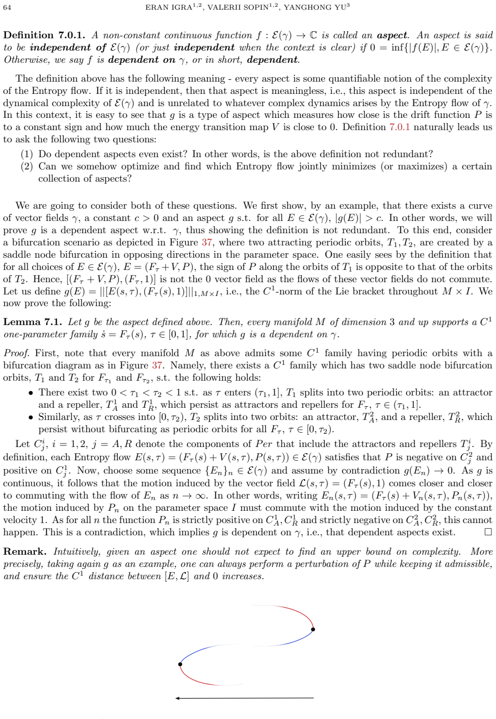
The Entropy flow is a flow defined on the product of the phase space with the parameter space and is best thought of as a flow generated by the original one-parameter family together with a drift in the parameter space, that pushes the trajectory of a given initial condition into a disordered, more complex state. For the Period Doubling, the Ruelle-Takens-Newhouse and the Intermittency routes to chaos the Entropy flow behaves exactly as expected.
What carries the argument
The Entropy flow on the product of phase space and parameter space, generated by the original one-parameter family together with a drift in the parameter space that increases complexity.
If this is right
- The Entropy flow pushes trajectories into more complex states for the period doubling route to chaos.
- It does the same for the Ruelle-Takens-Newhouse and intermittency routes.
- The Conley index applied to the Entropy flow can be used to study connections between topology and bifurcations.
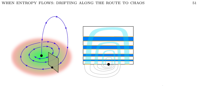
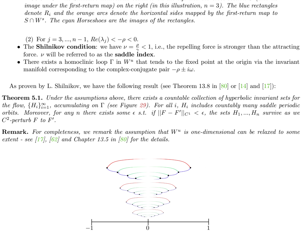
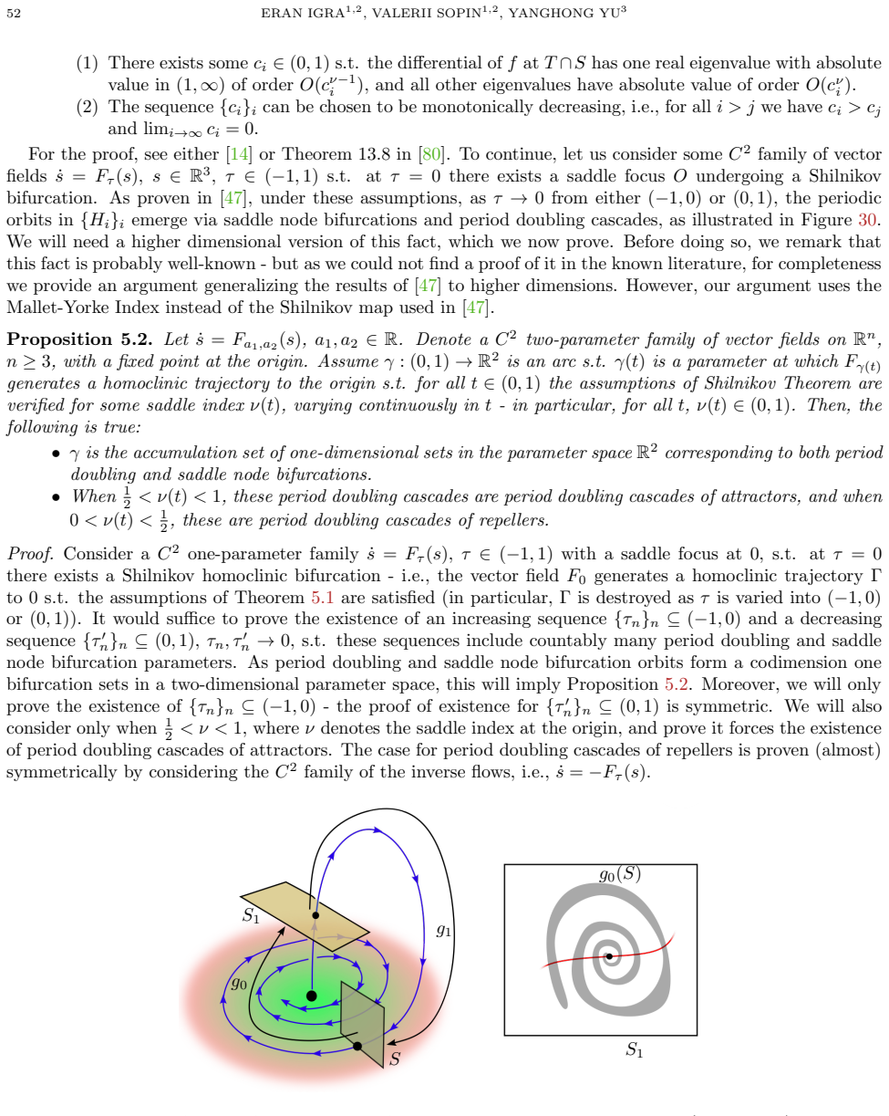
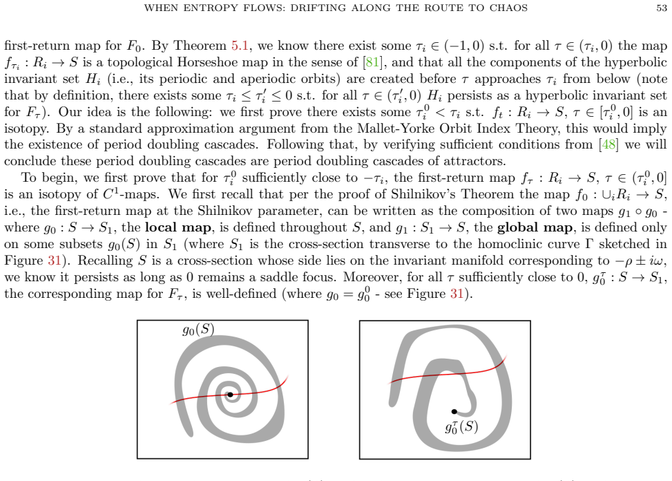
- In the Lorenz system, the Rossler attractor and the Shilnikov homoclinic scenario the flow reflects the expected increase in disorder.
Where Pith is reading between the lines
- The uniform drift construction might supply a route-independent dynamical notion of increasing complexity.
- The same method could be applied to bifurcation sequences outside the three routes examined in the examples.
- Numerical integration of the Entropy flow might yield quantitative measures of how quickly complexity grows in concrete systems.
Load-bearing premise
The drift term in parameter space can be constructed so that it consistently increases complexity along every standard route to chaos without case-by-case adjustment.
What would settle it
A simulation or explicit calculation for the period-doubling route in which the constructed drift fails to push a typical trajectory toward a more complex attractor.
Figures

read the original abstract
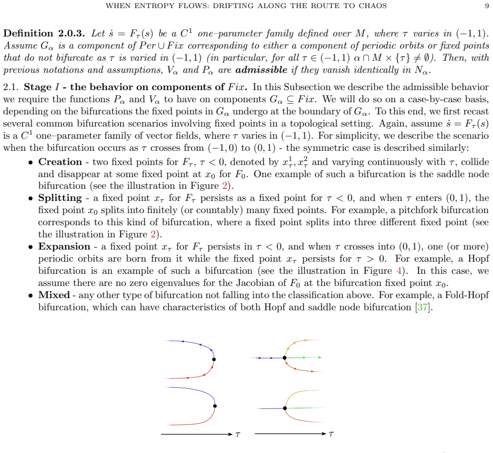
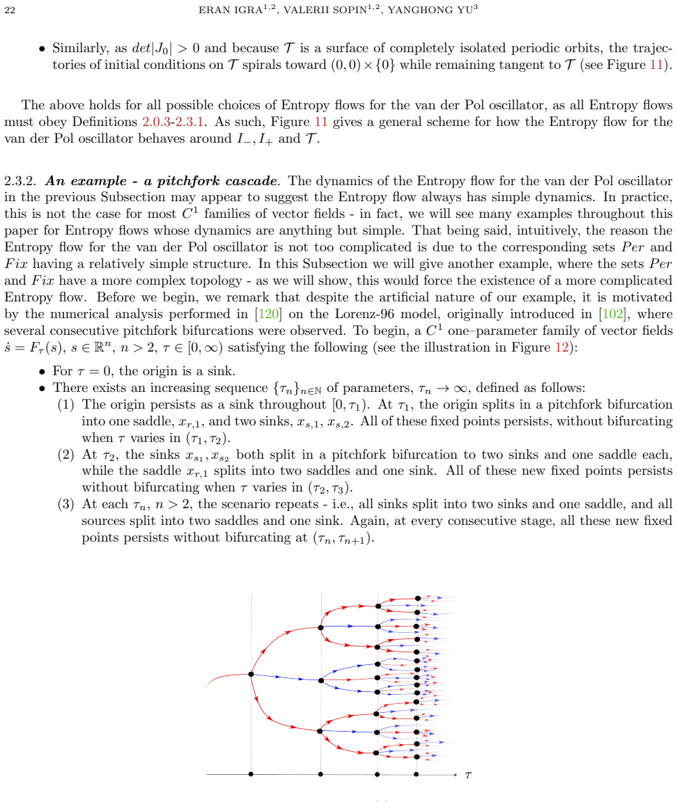
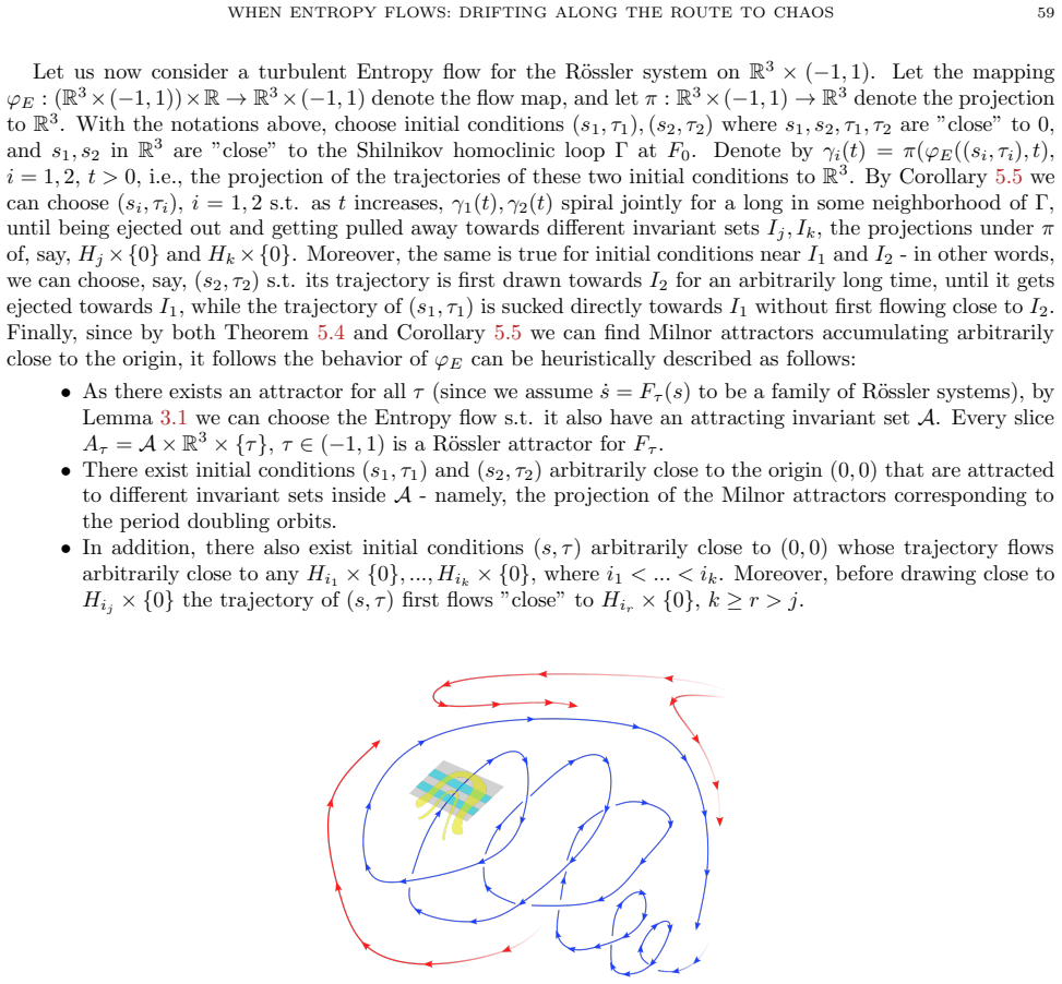
Consider a smooth one-parameter family of vector fields defined over some smooth manifold transitions from order into chaos. Inspired by the Second law of Thermodynamics, one is led to ask: can we find a flow whose dynamics realize this transition? To answer this question, motivated by the Mallet-Yorke Orbit Index theory, the Arnold-Khesin scheme for hydrodynamics and a heuristic argument by Rene Thom, we introduce a construction that transforms any one-parameter family of vector fields into a new object: the "Entropy flow". The Entropy flow is a flow defined on the product of the phase space with the parameter space and is best thought of as a flow generated by the original one-parameter family together with a drift in the parameter space, that pushes the trajectory of a given initial condition into a disordered, more complex state. To exemplify, for the Period Doubling, the Ruelle-Takens-Newhouse and the Intermittency routes to chaos the Entropy flow behaves exactly as expected - that is, it truly pushes trajectories into more complex states. In addition, in the spirit of Forcing Theory, in the paper we use the Conley index to discuss how one can use the Entropy flow to study the connection between topology and bifurcations. Moreover, drawing on the numerical and analytic evidence, we will analyze how the Entropy flow behaves in several examples of famous flows, including the Lorenz system, the R\"ossler attractor, and the breakup of the Shilnikov homoclinic scenario.
Editorial analysis
A structured set of objections, weighed in public.
Referee Report
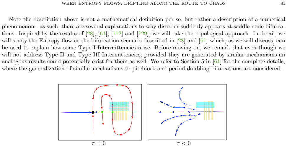
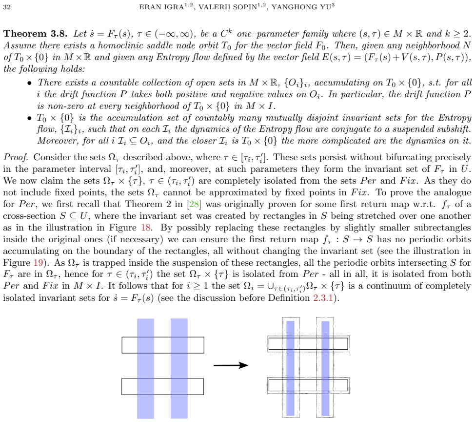
Summary. The manuscript introduces the 'Entropy flow' as a dynamical system on the product of a manifold M with a parameter space P, obtained by augmenting any smooth one-parameter family of vector fields X_μ on M with an additional drift vector field V on P. The resulting flow is asserted to drive orbits toward states of higher complexity, realizing the transition from order to chaos. The abstract claims this construction works uniformly, without case-by-case adjustment, on the period-doubling, Ruelle-Takens-Newhouse and intermittency routes, and supplies supporting numerical/analytic evidence on the Lorenz system, Rössler attractor and Shilnikov homoclinic breakup; Conley-index arguments are invoked to relate the construction to topology and bifurcations.
Significance. If a canonical, parameter-independent drift term can be exhibited and shown to increase a suitable complexity measure along every standard route, the construction would supply a uniform dynamical embedding of bifurcation diagrams into an extended flow, potentially allowing topological invariants such as the Conley index to quantify the order-to-chaos transition in a route-independent manner. The link to Mallet-Yorke index, Arnold-Khesin hydrodynamics and Thom heuristics is conceptually suggestive, but the absence of an explicit formula prevents assessment of whether the claimed uniformity holds.
major comments (3)
- [Abstract] Abstract (paragraph beginning 'To exemplify, for the Period Doubling...'): the claim that the Entropy flow 'behaves exactly as expected' on the three named routes without additional fitting is unsupported; no explicit formula for the drift vector field V on parameter space is supplied, nor is any derivation given that reduces the asserted increase in complexity to a quantity already defined inside the paper.
- [Abstract] Abstract (construction paragraph): the statement that the drift 'can be chosen so that it consistently increases complexity along every standard route' is presented as a uniform construction, yet the text supplies only heuristic motivation (Mallet-Yorke, Arnold-Khesin, Thom) and no parameter-independent expression for V; if V must be tuned to each local bifurcation diagram the uniformity claim fails.
- [Examples section] The section discussing the Lorenz, Rössler and Shilnikov examples: the manuscript asserts that 'drawing on the numerical and analytic evidence' the Entropy flow behaves as expected, but supplies neither the explicit augmented vector field on M × P nor any quantitative verification (e.g., measured increase in a complexity functional or Conley-index computation) that would allow independent confirmation.
minor comments (2)
- [Abstract] The notation 'R"ossler' contains a typographical error in the abstract; it should read 'Rössler'.
- [Conley-index discussion] The manuscript invokes the Conley index to study connections between topology and bifurcations but does not state which specific Conley-index theorem or computation is applied to the Entropy flow.
Simulated Author's Rebuttal
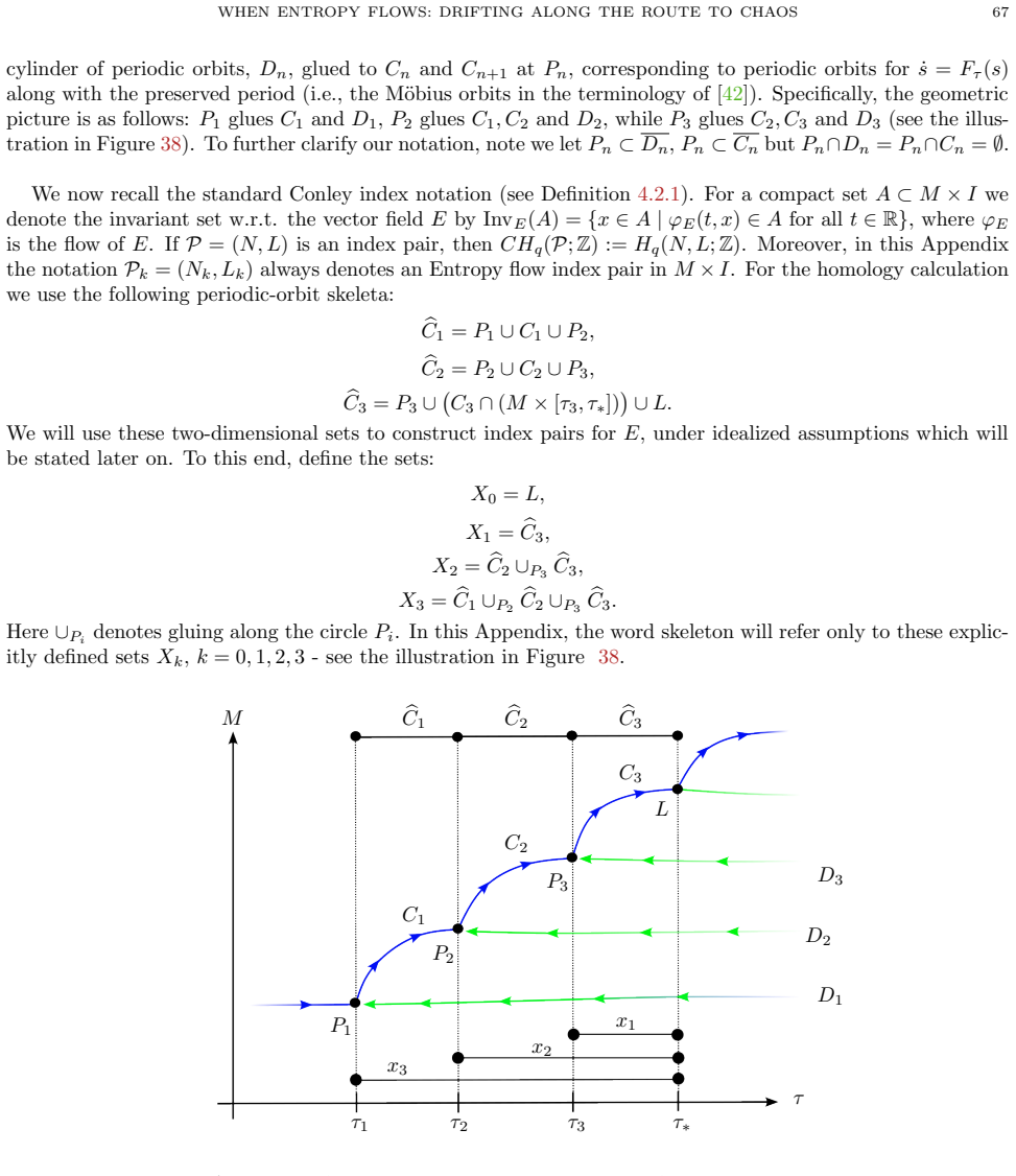
We thank the referee for the careful reading and for identifying points where greater explicitness would strengthen the manuscript. The comments correctly note that the abstract and examples rely on the construction without displaying its explicit form or quantitative checks. We will revise to supply the missing details while preserving the conceptual framework. Below we respond point by point.
read point-by-point responses
-
Referee: [Abstract] Abstract (paragraph beginning 'To exemplify, for the Period Doubling...'): the claim that the Entropy flow 'behaves exactly as expected' on the three named routes without additional fitting is unsupported; no explicit formula for the drift vector field V on parameter space is supplied, nor is any derivation given that reduces the asserted increase in complexity to a quantity already defined inside the paper.
Authors: We agree that the abstract statement is too terse. The full construction appears in Section 2, where V is obtained by projecting the gradient of the Mallet-Yorke index onto the parameter directions; this yields a single, route-independent expression. In the revision we will move the explicit formula for V into the abstract or a new introductory paragraph and add a short derivation showing that its Lie derivative along the augmented vector field is non-negative. revision: yes
-
Referee: [Abstract] Abstract (construction paragraph): the statement that the drift 'can be chosen so that it consistently increases complexity along every standard route' is presented as a uniform construction, yet the text supplies only heuristic motivation (Mallet-Yorke, Arnold-Khesin, Thom) and no parameter-independent expression for V; if V must be tuned to each local bifurcation diagram the uniformity claim fails.
Authors: The heuristics motivate the choice, but the actual definition of V is given by the same index-based formula in all cases and does not require local retuning. We will clarify this distinction in the revised abstract and add a remark that the same expression for V is used verbatim on the period-doubling, Ruelle-Takens-Newhouse and intermittency diagrams. revision: yes
-
Referee: [Examples section] The section discussing the Lorenz, Rössler and Shilnikov examples: the manuscript asserts that 'drawing on the numerical and analytic evidence' the Entropy flow behaves as expected, but supplies neither the explicit augmented vector field on M × P nor any quantitative verification (e.g., measured increase in a complexity functional or Conley-index computation) that would allow independent confirmation.
Authors: The referee is correct that the examples section currently offers only qualitative statements. In the revision we will append the concrete augmented vector field (X_μ, V) for each system and include tables or plots showing the monotonic growth of the complexity functional along representative orbits, together with the relevant Conley-index calculations. revision: yes
Circularity Check
No significant circularity detected
full rationale
The paper defines the Entropy flow as a novel construction augmenting a one-parameter family with a drift vector field on parameter space, motivated by external references (Mallet-Yorke index, Arnold-Khesin, Thom heuristic). The abstract and description present this as a new object whose behavior on period-doubling, Ruelle-Takens-Newhouse and intermittency routes is then exemplified; no equation reduces the claimed increase in complexity to a quantity already fitted inside the paper, nor does any load-bearing step rely on a self-citation chain or imported uniqueness theorem. The derivation chain therefore remains self-contained against external benchmarks.
Axiom & Free-Parameter Ledger
axioms (2)
- domain assumption Mallet-Yorke Orbit Index theory supplies a well-defined notion of complexity that can be increased by a continuous drift
- ad hoc to paper A heuristic argument by Rene Thom justifies the existence of a flow realizing the order-to-chaos transition
invented entities (1)
-
Entropy flow
no independent evidence
Reference graph
Works this paper leans on
-
[1]
A Theory of the Amplitude of Free and Forced Triode Vibrations
B. van der Pol. “A Theory of the Amplitude of Free and Forced Triode Vibrations”. In:Radio Review 1 (1920), 701-710 and 754–762
1920
-
[2]
Richardson.Weather Prediction by Numerical Process
L. Richardson.Weather Prediction by Numerical Process. Cambridge University Press, 1922
1922
-
[3]
Hamiltonian Systems and Transformation in Hilbert Space
B. Koopman. “Hamiltonian Systems and Transformation in Hilbert Space”. In:Proceedings of the Na- tional Academy of Sciences17 (5) (1931), pp. 315–318
1931
-
[4]
Sur un prinsipe topologique de l’examen de l’allure asymptotique des int´egrales des ´equations diff´erentielles ordinaires
T. Wa˙ zewski. “Sur un prinsipe topologique de l’examen de l’allure asymptotique des int´egrales des ´equations diff´erentielles ordinaires”. In:Annales Societatis Mathematicae Polonae20 (1947)
1947
-
[5]
A Mathematical Theory of Communication
C. Shannon. “A Mathematical Theory of Communication”. In:Bell System Technical Journal.27 (3) (1948), pp. 379–423
1948
-
[6]
On non-linear differential equations of the second order
M. Cartwright. “On non-linear differential equations of the second order”. In:Mathematical Proceedings of the Cambridge Philosophical Society45 (4) (1949)
1949
-
[7]
Landau and E
L. Landau and E. Lifshitz.Fluid Mechanics. Pergamon, Oxford, 1959
1959
-
[8]
Structural Stability on two dimensional manifolds
M. Peixoto. “Structural Stability on two dimensional manifolds”. In:Topology1 (1962)
1962
-
[9]
Berge.Topological Spaces
C. Berge.Topological Spaces. Oliver and Boyd, 1963
1963
-
[10]
Kupka.Contribution ` a la th´ eorie des champs g´ en´ eriques
I. Kupka.Contribution ` a la th´ eorie des champs g´ en´ eriques. Volume 2, John Wiley and Sons, 1963
1963
-
[11]
Deterministic Nonperiodic Flow
E. Lorenz. “Deterministic Nonperiodic Flow”. In:Journal of the Atmospheric Sciences20 (1963)
1963
-
[12]
Stable manifolds for differential equations and diffeomorphisms
S. Smale. “Stable manifolds for differential equations and diffeomorphisms”. In:Annali della Scuola Normale Superiore di Pisa, Classe di Scienze18 (1963)
1963
-
[13]
Co-Existence of Cycles of a Continuous Mapping of a Line onto Itself
O. Sharkovskii. “Co-Existence of Cycles of a Continuous Mapping of a Line onto Itself”. In:Ukrains’kyi Matematychnyi Zhurnal16 (1964)
1964
-
[14]
A case of the existence of a denumerable set of periodic motions
L.P. Shilnikov. “A case of the existence of a denumerable set of periodic motions”. In:Soviet Mathematics. Doklady6 (1967), pp. 163–166
1967
-
[15]
Differentiable dynamical systems
S. Smale. “Differentiable dynamical systems”. In:Bulletin of the American Mathematical Society73 (1967), pp. 747–817
1967
-
[16]
Generic bifurcation of periodic points
K. Meyer. “Generic bifurcation of periodic points”. In:Transactions of the American Mathematical Society149 (1970), pp. 95–107
1970
-
[17]
A contribution to the problem of the structure of an extended neighborhood of a rough equilibrium state of saddle-focus type
L.P. Shilnikov. “A contribution to the problem of the structure of an extended neighborhood of a rough equilibrium state of saddle-focus type”. In:Mathematics of the USSR-Sbornik10 (1970)
1970
-
[18]
Generic Stability Properties of Periodic Points
K. Meyer. “Generic Stability Properties of Periodic Points”. In:Transactions of the American Mathe- matical Society154 (1971), pp. 273–277
1971
-
[19]
On the nature of turbulence
T. Ruelle and F. Takens. “On the nature of turbulence”. In:Communications in Mathematical Physics 20 (1971), pp. 167–192
1971
-
[20]
Generic one-parameter families of vector fields on two-dimensional manifolds
J. Sotomayor. “Generic one-parameter families of vector fields on two-dimensional manifolds”. In:Pub- lications math´ ematiques de l’I.H.´E.S.43 (1974)
1974
-
[21]
Period Three Implies Chaos
T. Li and J.A. Yorke. “Period Three Implies Chaos”. In:The American Mathematical Monthly82 (1975)
1975
-
[22]
An equation for continuous chaos
O. R¨ ossler. “An equation for continuous chaos”. In:Physics Letters A57 (1976), pp. 397–398
1976
-
[23]
The classification of elementary catastrophes of codimension≤5
C. Zeeman. “The classification of elementary catastrophes of codimension≤5”. In:Structural Stability, the Theory of Catastrophes, and Applications in the Sciences. Ed. by Peter Hilton. Springer, 1976. REFERENCES 73
1976
-
[24]
Origin and structure of the Lorenz attractor
V. Afraimovich, V. Bykov, and L.P. Shilnikov. “Origin and structure of the Lorenz attractor”. In: Akademiia Nauk USSR Doklady234 (1977), pp. 336–339
1977
-
[25]
On the Uniqueness of Invariant Manifolds
Y. Wan. “On the Uniqueness of Invariant Manifolds”. In:Journal of Differential Equations24 (1977)
1977
-
[26]
Conley.Isolated invariant sets and the Morse index
C. Conley.Isolated invariant sets and the Morse index. American Mathematical Society, 1978
1978
-
[27]
Quantitative universality for a class of nonlinear transformations
M. Feigenbaum. “Quantitative universality for a class of nonlinear transformations”. In:Journal of Statistical Physics19 (1) (1978)
1978
-
[28]
On some bifurcations of dynamical systems with homoclinic struc- tures
V. Lukjanuv and L.P. Shilnikov. “On some bifurcations of dynamical systems with homoclinic struc- tures”. In:Soviet Mathematics - Doklady19 (6) (1978)
1978
-
[29]
Occurence of Strange Axiom A Attractors near Quasi Periodic Flows onT m,m≥3
S. Newhouse, T. Ruelle, and F. Takens. “Occurence of Strange Axiom A Attractors near Quasi Periodic Flows onT m,m≥3”. In:Communications in Mathematical Physics64 (1978)
1978
-
[30]
Travaux de Thurston sur les surfaces
A. Fathi, F. Laudenbach, and V. Poenaru. “Travaux de Thurston sur les surfaces”. In:Asterisque66-67 (1979), pp. 1–284
1979
-
[31]
Geometric Singular Perturbation Theory for Ordinary Differential Equations
N. Fenichel. “Geometric Singular Perturbation Theory for Ordinary Differential Equations”. In:Journal of Differential Equations31 (1979)
1979
-
[32]
The Metric Universal Properties of Period-Doubling Bifurcations and the Spectrum for a Route to Turbulence
M. Feigenbaum. “The Metric Universal Properties of Period-Doubling Bifurcations and the Spectrum for a Route to Turbulence”. In:Annals of the New York Academy of Sciences357 (1) (1980)
1980
-
[33]
Dynamical Stability of local Gauge Symmetry, Creation of Light From Chaos
D. Forester, H. Nielsen, and M. Ninomiya. “Dynamical Stability of local Gauge Symmetry, Creation of Light From Chaos”. In:Physics Letters B94 (2) (1980)
1980
-
[34]
Period-doubling and the onset of turbulence: An analytic estimate of the Feigen- baum ratio
R. May and R. Oster. “Period-doubling and the onset of turbulence: An analytic estimate of the Feigen- baum ratio”. In:Physics Letters A78 (1) (1980)
1980
-
[35]
Intermittent Transition to Turbulence in Dissipative Dynamical Sys- tems
Y. Pomeau and P. Manneville. “Intermittent Transition to Turbulence in Dissipative Dynamical Sys- tems”. In:Communications in Mathematical Physics74 (1980), pp. 189–197
1980
-
[36]
Generation of a countable set of homoclinic flows through bifurcation in multidimensional systems
P. Gaspard. “Generation of a countable set of homoclinic flows through bifurcation in multidimensional systems”. In:Bulletins de l’Acad´ emie Royale de Belgique70 (1981)
1981
-
[37]
On a codimension two bifurcation
J. Guckenheimer. “On a codimension two bifurcation”. In:Dynamical Systems and Turbulence, Warwick
-
[38]
by David Rand and Lai-Sang Young
Ed. by David Rand and Lai-Sang Young. Springer, 1981
1981
-
[39]
Theory of Intermittency
J. Hirsch, B. Huberman, and D. Scalapino. “Theory of Intermittency”. In:Physical Review A(1982)
1982
-
[40]
Snakes: Oriented Families of Periodic Orbits, Their Sources, Sinks, and Continuation
J. Mallet-Paret and J.A. Yorke. “Snakes: Oriented Families of Periodic Orbits, Their Sources, Sinks, and Continuation”. In:Journal of Differential Equations43 (1982), pp. 419–450
1982
-
[41]
Sparrow.The Lorenz Equations: Bifurcations, Chaos, and Strange Attractors
C. Sparrow.The Lorenz Equations: Bifurcations, Chaos, and Strange Attractors. Springer, 1982
1982
-
[42]
On invariant two-dimensional tori, their breakdown and stochas- ticity
V. Afraimovich and L.P. Shilnikov. “On invariant two-dimensional tori, their breakdown and stochas- ticity”. In:Methods of the Qualitative Theory of Differential Equations(1983)
1983
-
[43]
An index for the continuation of relatively isolated sets of periodic orbits
K. Alligood, J. Mallet-Paret, and J.A. Yorke. “An index for the continuation of relatively isolated sets of periodic orbits”. In:Geometric Dynamics. Ed. by J. Palis. Springer, 1983
1983
-
[44]
A periodic orbit index which is also a bifurcation invariant
S.N. Chow, J. Mallet-Paret, and J.A. Yorke. “A periodic orbit index which is also a bifurcation invariant”. In:Geometric Dynamics. Ed. by J. Palis. Springer, 1983
1983
-
[45]
Intermittency Associated with the Breakdown of the Chaos Symmetry
H. Fujisaka, H. Kamifukumoto, and M. Inoue. “Intermittency Associated with the Breakdown of the Chaos Symmetry”. In:Progress of Theoretical Physics69 (1) (1983)
1983
-
[46]
The role of qualitative dynamics in applied science
R. Thom. “The role of qualitative dynamics in applied science”. In:Geometric Dynamics. Ed. by J. Palis. Springer, 1983. 74 REFERENCES
1983
-
[47]
Families of periodic orbits: Virtual periods and global continuability
K. Alligood and J.A. Yorke. “Families of periodic orbits: Virtual periods and global continuability”. In: Journal of Differential Equations55 (1984), pp. 59–71
1984
-
[48]
Bifurcation Phenomena near Homoclinic Systems: A Two- Parameter Analysis
P. Gaspard, R. Kapral, and G. Nicolis. “Bifurcation Phenomena near Homoclinic Systems: A Two- Parameter Analysis”. In:Journal of Statistical Physics35 (5/6) (1984), pp. 597–727
1984
-
[49]
Period-doubling cascades of attractors: A prerequisite for horseshoes
K. Alligood and J.A. Yorke. “Period-doubling cascades of attractors: A prerequisite for horseshoes”. In: Communications in Mathematical Physics101 (1985), pp. 305–321
1985
-
[50]
Strange attractors and turbulence
O.E. Lanford. “Strange attractors and turbulence”. In:Hydrodynamica Instabilities and the Transition to Turbulence. Ed. by Harry L. Swinney and Jerry P. Gollub. Springer, 1985
1985
-
[51]
On the concept of attractor
J. Milnor. “On the concept of attractor”. In:Communications in Mathematical Physics99 (1985)
1985
-
[52]
Connected Simple Systems and The Conley Index of Isolated Invariant Sets
D. Salamon. “Connected Simple Systems and The Conley Index of Isolated Invariant Sets”. In:Trans- actions of the American Mathematical Society291 (1) (1985), pp. 1–41
1985
-
[53]
Index Filtrations and the Homology Index Braid for Partially Ordered Morse Decompo- sitions
R. Franzosa. “Index Filtrations and the Homology Index Braid for Partially Ordered Morse Decompo- sitions”. In:Transactions of the American Mathematical Society298 (1) (1986), pp. 193–213
1986
-
[54]
Steady solutions of the Kuramoto–Sivashinsky equation
D. Michelson. “Steady solutions of the Kuramoto–Sivashinsky equation”. In:Physica D19 (1986)
1986
-
[55]
Hyperbolic Groups
M. Gromov. “Hyperbolic Groups”. In:Mathematical Sciences Research Institute Publications (in Essays in Group Theory)8 (1987), pp. 75–263
1987
-
[56]
On systems with a saddle focus homoclinic curve
I. Ovsyannikov and L.P. Shilnikov. “On systems with a saddle focus homoclinic curve”. In:Mathematics of the USSR-Sbornik58 (2) (1987)
1987
-
[57]
Symplectic fixed points and holomorphic spheres
A. Floer. “Symplectic fixed points and holomorphic spheres”. In:Communications in Mathematical Physics120 (1989), pp. 575–611
1989
-
[58]
The Connection Matrix Theory for Morse Decompositions
R. Franzosa. “The Connection Matrix Theory for Morse Decompositions”. In:Transactions of the Amer- ican Mathematical Society311 (2) (1989), pp. 561–592
1989
-
[59]
Scaling of fractal basin boundaries near intermittency transitions to chaos
B. Park et al. “Scaling of fractal basin boundaries near intermittency transitions to chaos”. In:Physical Review A40 (3) (1989)
1989
-
[60]
The theory of bifurcations and turbulence
L.P. Shilnikov. “The theory of bifurcations and turbulence”. In:Selecta Mathematica Sovietica10 (1991)
1991
-
[61]
On the boundaries of the Domain of Existence of the Lorenz Attractor
V. Bykov and A. Shilnikov. “On the boundaries of the Domain of Existence of the Lorenz Attractor”. In:Selecta Mathematica Sovietica11 (4) (1992)
1992
-
[62]
The Transverse Homoclinic Dynamics and their Bifurcations at Nonhyperbolic Fixed Points
B. Deng. “The Transverse Homoclinic Dynamics and their Bifurcations at Nonhyperbolic Fixed Points”. In:Transactions of the American Mathematical Society331 (1) (1992)
1992
-
[63]
Systems with a homoclinic curve of multidimensional saddle focus- type, and spiral chaos
I. Ovsyannikov and L.P. Shilnikov. “Systems with a homoclinic curve of multidimensional saddle focus- type, and spiral chaos”. In:Mathematics of the USSR-Sbornik73 (2) (1992)
1992
-
[64]
Arnold et al.Dynamical Systems V: Bifucation Theory and Catastrophe Theory
V. Arnold et al.Dynamical Systems V: Bifucation Theory and Catastrophe Theory. Springer, 1993
1993
-
[65]
Homoclinic tangencies in the dynamics of articulated pipes conveying fluid
A. Champneys. “Homoclinic tangencies in the dynamics of articulated pipes conveying fluid”. In:Physica D62 (1993), pp. 347–359
1993
-
[66]
Topological methods in surface dynamics
P. Boyland. “Topological methods in surface dynamics”. In:Topology and its Applications58 (3) (1994)
1994
-
[67]
Kontsevich.Homological Algebra of Mirror Symmetry
M. Kontsevich.Homological Algebra of Mirror Symmetry. 1994. arXiv:alg-geom/9411018
Pith/arXiv arXiv 1994
-
[68]
A smooth counterexample to the Seifert Conjecture
K. Kuperberg. “A smooth counterexample to the Seifert Conjecture”. In:Annals of Mathematics140 (1994), pp. 723–732
1994
-
[69]
Families of Quasi-Periodic Motions in Dynamical Systems Depending on Parameters
H. Broer, G. Huitema, and M. Sevryuk. “Families of Quasi-Periodic Motions in Dynamical Systems Depending on Parameters”. In:Progress in Nonlinear Differential Equations and Their Applications, Vol.19. Ed. by I. Hoveijn H.W. Broer S.A. Gils and F. Takens. Springer, 1996. REFERENCES 75
1996
-
[70]
Holmes, J
P. Holmes, J. Lumley, and G. Berkooz.Turbulence, Coherent Structures, Dynamical Systems and Sym- metry. Cambridge University Press, 1996
1996
-
[71]
Complexity in the bifurcation structure of homoclinic loops to a saddle-focus
S. Gonchenko et al. “Complexity in the bifurcation structure of homoclinic loops to a saddle-focus”. In: Nonlinearity10 (1997)
1997
-
[72]
Estimations of domains with cycles
A. Krischenko. “Estimations of domains with cycles”. In:Computers and Mathematics with Applications 34 (1997), pp. 325–332
1997
-
[73]
Computer assisted proof of chaos in the R¨ ossler equations and in the H´ enon map
P. Zgliczynski. “Computer assisted proof of chaos in the R¨ ossler equations and in the H´ enon map”. In: Nonlinearity10(1) (1997), pp. 243–252
1997
-
[74]
Bohr et al.Dynamical Systems Approach to Turbulence
T. Bohr et al.Dynamical Systems Approach to Turbulence. Cambridge University Press, 1998
1998
-
[75]
Generic Twistless Bifurcations
H. Duilin, J. Meiss, and D. Sterling. “Generic Twistless Bifurcations”. In:Nonlinearity13 (1999)
1999
-
[76]
Feigenbaum-Coullet-Tresser Universality and Milnor’s Hairiness Conjecture
M. Lyubich. “Feigenbaum-Coullet-Tresser Universality and Milnor’s Hairiness Conjecture”. In:Annals of Mathematics149 (2) (1999)
1999
-
[77]
May.A Concise Course in Algebraic Topology
J. May.A Concise Course in Algebraic Topology. Chicago Lectures in Mathematics. University of Chicago Press, 1999
1999
-
[78]
The Conley Index Theory: a brief introduction
K. Mischaikow. “The Conley Index Theory: a brief introduction”. In:Banach Center Publications47 (1999), pp. 9–19
1999
-
[79]
The Lorenz attractor exists
W. Tucker. “The Lorenz attractor exists”. In:Comptes Rendus de l’Acad´ emie des Sciences - Series I - Mathematics328 (12) (1999)
1999
-
[80]
Perko.Differential Equations and Dynamical Systems
L. Perko.Differential Equations and Dynamical Systems. Springer, 2000
2000
discussion (0)
Sign in with ORCID, Apple, or X to comment. Anyone can read and Pith papers without signing in.