Universal Inference for model selection on networks
Pith reviewed 2026-07-01 00:56 UTC · model grok-4.3
The pith
Edge sampling produces an e-value that controls type I error in finite samples for network hypothesis tests.
A machine-rendered reading of the paper's core claim, the machinery that carries it, and where it could break.
Core claim
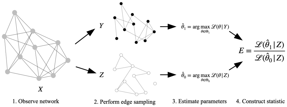
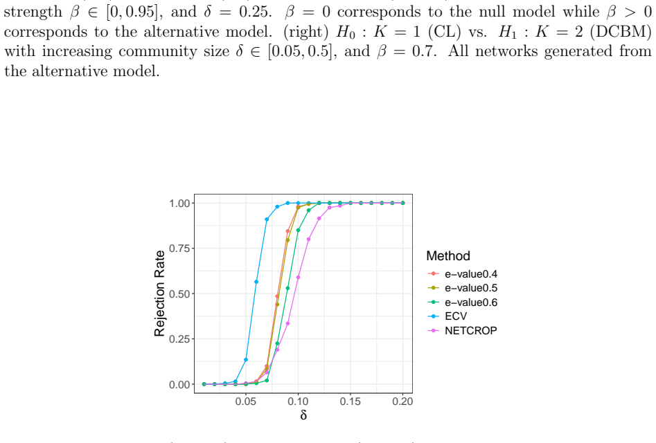
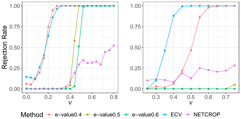
By using edge sampling to obtain two networks with tractable dependence, the authors construct a Universal Inference statistic that is an e-value. This provides finite-sample type I error control under nearly any hypothesis test on networks. The log of the test statistic diverges to positive infinity under various alternative models. The procedure performs well for selecting random graph models and the number of communities on both simulated and real-world networks.
What carries the argument
The e-value constructed via Universal Inference on edge-sampled dependent network splits.
If this is right
- Finite-sample type I error control holds for a wide range of network hypothesis tests.
- The method applies directly to selecting among random graph models.
- It can be used to choose the number of communities in a network.
- The log statistic diverges under various alternative models, supporting consistency.
Where Pith is reading between the lines
- The edge-splitting idea could extend to other single-observation dependent structures such as spatial or temporal data.
- It might reduce reliance on bootstrap or permutation methods when testing network models.
- Optimal edge-sampling fractions or power analysis could be explored as follow-on questions.
Load-bearing premise
Edge sampling must produce two networks whose dependence structure still permits construction of a valid e-value under the Universal Inference framework without invalidating finite-sample type I error control.
What would settle it
A simulation study or real network dataset under a known null where the proposed statistic exceeds the critical threshold more frequently than the nominal level, or fails to diverge under a specified alternative.
Figures
read the original abstract
Model selection and hypothesis testing are important tasks on networks. A key challenge lies in the inherent dependence in network data, as well as the fact that typically only a single realization is observed. As a result, many existing methods must be carefully tailored to specific models and only come with asymptotic theoretical guarantees. In this work, however, we propose a general model selection framework using Universal Inference, making our method widely applicable to various testing scenarios. Since Universal Inference requires two sets of data, we employ edge sampling to obtain proper networks with tractable dependence. We prove that the proposed statistic is an e-value, thus controlling the type I error rate in finite samples under nearly any hypothesis test. To our knowledge, this is the first Universal Inference-type statistic constructed from dependent splits of data as well as the first finite-sample testing guarantee for hypothesis testing on networks. We also prove that the logarithm of the test statistic diverges to positive infinity under various alternative models. On simulated and real-world networks, the proposed method performs well on tasks such as choosing the random graph model and the number of communities.
Editorial analysis
A structured set of objections, weighed in public.
Referee Report
Summary. The paper proposes a Universal Inference framework for model selection and hypothesis testing on networks. It uses edge sampling to split a single observed network into two dependent networks with tractable dependence structure, constructs a test statistic, and claims to prove that this statistic is an e-value (thus guaranteeing finite-sample type I error control for nearly any hypothesis test). It further claims to prove that the log of the statistic diverges to +∞ under various alternatives, and demonstrates the method on simulated and real networks for tasks such as random graph model selection and choosing the number of communities. The work positions itself as the first Universal Inference statistic from dependent splits and the first finite-sample guarantee for network hypothesis testing.
Significance. If the central proofs hold, the result would be significant: it supplies the first finite-sample type I error control for network model selection and testing (where only a single realization is typically observed and most existing methods are asymptotic or model-specific). The explicit construction of an e-value from edge-sampled dependent splits extends the Universal Inference framework in a non-trivial way, and the divergence result under alternatives provides a power guarantee. These elements, if substantiated by the derivations, would be a clear methodological advance in statistical network analysis.
major comments (2)
- [Proof of e-value property (likely §3 or Theorem 1)] The central claim that the proposed statistic is an e-value (and thus controls type I error in finite samples) rests on the edge-sampling construction preserving the necessary martingale or supermartingale property under the dependence induced by sampling edges from a single network. The abstract asserts this result, but the explicit verification that the dependence between the two splits does not invalidate the e-value property under the Universal Inference framework is load-bearing and must be shown in detail (e.g., in the section containing the main theorem).
- [Divergence result under alternatives (likely §4)] The claim that log of the test statistic diverges to +∞ under alternatives likewise depends on the edge-sampling probability and the specific form of the alternative; the paper must state the precise conditions on the alternative models and sampling rate under which divergence holds, otherwise the power guarantee is not fully established.
minor comments (2)
- Clarify the precise class of hypothesis tests to which the finite-sample guarantee applies (the phrase 'nearly any hypothesis test' in the abstract is vague).
- Define the edge-sampling probability parameter at the first appearance and use consistent notation throughout.
Simulated Author's Rebuttal
We thank the referee for their careful reading of the manuscript and for the constructive comments on the central theoretical claims. We address each major comment below and indicate the revisions that will be made to strengthen the presentation.
read point-by-point responses
-
Referee: [Proof of e-value property (likely §3 or Theorem 1)] The central claim that the proposed statistic is an e-value (and thus controls type I error in finite samples) rests on the edge-sampling construction preserving the necessary martingale or supermartingale property under the dependence induced by sampling edges from a single network. The abstract asserts this result, but the explicit verification that the dependence between the two splits does not invalidate the e-value property under the Universal Inference framework is load-bearing and must be shown in detail (e.g., in the section containing the main theorem).
Authors: We appreciate the referee's emphasis on the need for explicit verification of the e-value property. The proof appears in Section 3 and Theorem 1, where we establish that the edge-sampling split preserves the required supermartingale property by computing the conditional expectation of the likelihood ratio under the induced dependence and showing it is at most 1 under the null. To make this verification more detailed and self-contained as requested, we will expand the proof in the revised manuscript with an additional lemma that explicitly bounds the effect of the dependence between the two sampled networks and confirms the property holds for any fixed sampling probability in (0,1). revision: yes
-
Referee: [Divergence result under alternatives (likely §4)] The claim that log of the test statistic diverges to +∞ under alternatives likewise depends on the edge-sampling probability and the specific form of the alternative; the paper must state the precise conditions on the alternative models and sampling rate under which divergence holds, otherwise the power guarantee is not fully established.
Authors: We agree that the conditions for the divergence result should be stated with greater precision. Section 4 proves that the log-statistic diverges to +∞ under alternatives in which the two models differ in their edge-probability parameters (for Erdős–Rényi and configuration models) or in community structure (for stochastic block models), with the edge-sampling probability held fixed in (0,1) and network size n → ∞. In the revision we will add an explicit statement of these conditions at the start of Section 4, including the precise requirements on the parameter separation and the sampling rate, to make the power guarantee fully transparent. revision: yes
Circularity Check
No significant circularity; derivation is a proof on external UI framework
full rationale
The paper's central result is a proof that an e-value can be constructed from edge-sampled dependent network splits while preserving finite-sample type I error control under the Universal Inference framework. This is presented as a mathematical construction and proof building on external theory (Universal Inference), with no equations or steps shown that reduce the claimed e-value property or divergence result to a fitted parameter, self-defined quantity, or load-bearing self-citation by construction. The abstract and description indicate the result is derived rather than assumed or renamed from inputs. No steps match the enumerated circularity patterns.
Axiom & Free-Parameter Ledger
axioms (1)
- standard math Standard properties of e-values under the Universal Inference framework
Reference graph
Works this paper leans on
-
[1]
Adamic, L. A. and Glance, N. (2005). The political blogosphere and the 2004 us election: divided they blog. InProceedings of the 3rd international workshop on Link discovery, pages 36–43. Ancell, E., Witten, D., and Kessler, D. (2025). Post-selection inference with a single real- ization of a network.arXiv preprint arXiv:2508.11843. Bhadra, S., Tang, M., ...
arXiv 2005
-
[2]
and Newman, M
18 Karrer, B. and Newman, M. E. J. (2011). Stochastic blockmodels and community structure in networks.Physical Review E, 83:016107. Lei, J. and Rinaldo, A. (2015). Consistency of spectral clustering in sparse stochastic block models.Annals of Statistics, 43(1):215–237. Leiner, J., Duan, B., Wasserman, L., and Ramdas, A. (2025). Data fission: splitting a s...
2011
-
[3]
Rohe, K., Chatterjee, S., and Yu, B. (2011). Spectral clustering and the high-dimensional stochastic blockmodel.The Annals of Statistics, 39(4):1878–1915. Sengupta, S. and Chen, Y. (2018). A block model for node popularity in networks with com- munity structure.Journal of the Royal Statistical Society: Series B (Statistical Methodol- ogy), 80(2):365–386. ...
arXiv 2011
-
[4]
Proof.Assume thatA∼P(θ ∗) whereθ ∗ ∈Θ 0, i.e., the network was generated under the null hypothesis
Under A1 and for anyn, the statistic constructed in Section 3.1 is an e-value i.e., sup θ∈Θ0 EθE≤1. Proof.Assume thatA∼P(θ ∗) whereθ ∗ ∈Θ 0, i.e., the network was generated under the null hypothesis. Then Eθ∗ ( L( γ 1−γ P(ˆθ1)|Z) L(P(ˆθ0)|Z) ) ≤E θ∗ ( L( γ 1−γ P(ˆθ1)|Z) L(γP(θ ∗)|Z) ) where ˆθ1 = arg max θ∈Θ1 L(θ|Y) since ˆθ0 = arg max θ∈Θ0 L(θ|Z) such th...
2020
-
[5]
27 Proof.We have that Xn = X ij {Pij(ˆθ)−ϱ nPij(θ∗)}= X ij (Aij −EA ij) since Sengupta and Chen (2018) show that A1 is met for the PABM
asn→ ∞for some constantk, and, hence,X n =o p(ϱnn2). 27 Proof.We have that Xn = X ij {Pij(ˆθ)−ϱ nPij(θ∗)}= X ij (Aij −EA ij) since Sengupta and Chen (2018) show that A1 is met for the PABM. The terms inside the sum are clearly independent with mean 0 and (finite) varianceϱ nPij(θ∗){1−ϱ nPij(θ∗)}such that s2 n = X ij ϱnPij(θ∗){1−ϱ nPij(θ∗)}=O(ϱ nn2). We wa...
2018
-
[6]
are easy to deduce as this model is a special case of the PABM. We start by defining ˆλik(ˆc) = Pn j=1 Yij1(ˆcj =k) {P ab Yab1(ˆca = ˆci,ˆcb =k)} 1/2 =O p(ϱ1/2 n ) (2) and λ∗ ik(ˆc) = Pn j=1 Pij(θ∗)1(ˆcj =k) {P ab Pab(θ∗)1(ˆca = ˆci,ˆcb =k)} 1/2 where ˆcis a function ofYand Sengupta and Chen (2018) show that the MLEs of the PABM take the form in (2). We t...
2018
-
[7]
We next note that there could be an identifiability problem betweenˆcandc ∗, i.e., community ‘1’ in ˆccould be different from community ‘1’ inc ∗
First, by Lemma 1, for any ϵ1 >0, P(X(1) n ≤ −ϵ1ϱnn2)→0. We next note that there could be an identifiability problem betweenˆcandc ∗, i.e., community ‘1’ in ˆccould be different from community ‘1’ inc ∗. For notational simplicity, we assume that ˆcandc ∗ are “aligned” such that community labels correspond to the same blocks. Now, we separate the probabili...
1998
-
[8]
ϱnPij(θ∗) ( 1− ϱn¯p ϱnPij(θ∗) 1/2)#! = exp
Proof.We start by writing outX n as Xn = X ij Aij log ϱnPij(θ∗) ϱn¯p Recall thatA ij ind. ∼Bernoulli(ϱ nPij(θ∗)). IfY∼Bernoulli(θ), then the moment generating function,M Y (t), is MY (t) =Ee Y t = 1−θ+θe t. Moreover, the moment generating function ofαYwhereαis a constant is MαY (t) =Ee (αY)t =M Y (αt) = 1−θ+θe αt. 33 Additionally, ifY 1, . . . , Ym are in...
2020
-
[9]
ThenE(logE n) =−∞
where0< θ 0 <1. ThenE(logE n) =−∞. Proof.From Wasserman et al. (2020), we splitX 1, . . . , X2n into two partsD 0 andD
2020
-
[10]
shortcut
Proof.First, we can replace P ij Aij in the denominator of ˆψi with ¯pϱnn2 where ¯p= 1 n2 X ij Pij(θ∗) as a “shortcut” since this term converges much faster than other appropriately scaled random variables. This assumption has been previously made in the literature (Yanchenko et al., 2025). Then we can writeX n as Xn = X ij Aij log ϱn ˜ψ∗ i ˜ψ∗ j ˆψi ˆψj ...
2025
-
[11]
merging operator
Proof.We start by writing outX n as Xn = X ij Aij log ϱnPij(θ∗) ϱn ˜ψ∗ i ˜ψ∗ j ! Similar to the proof of Lemma 5, we use a Chernoff bound argument and find P(Xn ≤ϵϱ nn2)≤exp ¯pϱnn2 " ϵ 2¯p− 1 ¯pn2 X ij Pij(θ∗)− { ˜ψ∗ i ˜ψ∗ j Pij(θ∗)}1/2 #! . Additionally, X ij ˜ψ∗ i ˜ψ∗ j = 1 ¯pn2 X ijkℓ Pik(θ∗)Pjℓ(θ∗) = 1 ¯pn2 X ik Pik(θ∗) ! X jℓ Pjℓ(θ∗) ! = ¯pn2 = X ij ...
2017
-
[12]
Proof.First, Xn =− X ij Aij(log ˆB˜c∗ i ,˜c∗ j −logϱ n ˜B∗ ˜c∗ i ,˜c∗ j ) 41 Then, P(Xn ≤ −ϵϱ nn2)≤P(|X n| ≥ϵϱ nn2). We write the (scaled) absolute value as |Xn| ϱnn2 ≤ 1 ϱnn2 X ij Aij|log ˆB˜c∗ i ,˜c∗ j −logϱ n ˜B∗ ˜c∗ i ,˜c∗ j |= K−1X k=1 K−1X ℓ=1 Skℓ ϱnn2 log ˆBkℓ ϱn ˜B∗ kℓ ∼ K−1X k=1 K−1X ℓ=1 ˆBkℓ ϱn log ˆBkℓ/ϱn ˜B∗ kℓ where Skℓ = X ij Aij1(˜c∗ i =k,˜...
2017
-
[13]
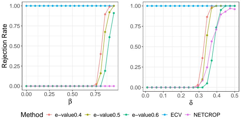
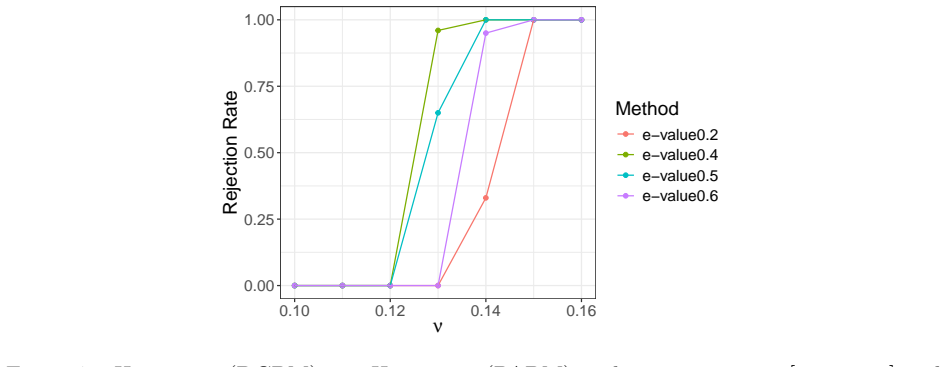
S7 Additional simulation results: DCBM versus PABM We provide an additional simulation setting to demonstrate the flexibility of the proposed method
All networks are generated under the alternative model. S7 Additional simulation results: DCBM versus PABM We provide an additional simulation setting to demonstrate the flexibility of the proposed method. Similar to the SBM vs. DCBM test, we test two models which both exhibit com- munity structure but have different levels of flexibility. Namely, we test...
2018
discussion (0)
Sign in with ORCID, Apple, or X to comment. Anyone can read and Pith papers without signing in.