AU or pc? Inferring the distance of magnetized plasma near FRBs from propagation diagnostics
Reviewed by Pith T0 review T1 audit T2 compute T3 formal T4 kernel 2026-07-07 19:34 UTCglm-5.2pith:Y6VUQYSUrecord.jsonopen to challenge →
The pith
Three propagation signals pin FRB environments to AU or pc scales
A machine-rendered reading of the paper's core claim, the machinery that carries it, and where it could break.
Core claim
The central object is the source-to-magneto-active-screen distance D_B, derived by combining temporal scattering, depolarization width sigma_RM, and RM variation rate |dRM/dt| into a single geometric closure. The key finding is that this combination of three measurable propagation effects suffices to estimate the physical scale of an FRB's magnetized environment at order-of-magnitude level without assuming whether the environment is a binary companion wind or a supernova remnant. The application to six repeaters reveals a genuine diversity: some sources sit at AU scales consistent with binary separations, others at parsec scales consistent with SNR shells, and the assignment can flip between
What carries the argument
Eq. 8 (co-located screen and magneto-active region): D_B ~ 415 AU * (sigma_RM/10 rad m^-2)^2 * (tau_scat/1 ms)^-1 * (|dRM/dt|/10 rad m^-2 day^-1)^-2 * (v/100 km/s)^2, with D_S/D_B ~ 1. Eq. 7 (spatially separated screen): D_B ~ 0.45 pc * (sigma_RM/10)^2 * (tau_scat/1 ms)^-1/2 * (|dRM/dt|/10)^-1 * (v/100 km/s) * sqrt(D_S/100 pc). The log-linear consistency check (Eq. 15) predicts a slope-unity relation between sqrt(tau_scat)|RM| and sigma_RM under a single-class origin; the observed slope is 0.31 +/- 0.19, shallower than unity but consistent within scatter.
If this is right
- If the co-location assumption holds, the AU-vs-pc split among repeaters directly distinguishes binary-companion environments from supernova-remnant environments, constraining FRB progenitor channels.
- Simultaneous wideband measurements of scattering, depolarization, and RM from upcoming instruments (CHORD, DSA) could reduce the current order-of-magnitude uncertainties to factor-of-few, enabling model discrimination for individual sources.
- Independent scintillation-based screen-distance measurements (e.g., from interstellar scintillation) would provide an external anchor for D_S, directly testing whether the scattering and Faraday-active regions are physically associated.
- If future data show the log-linear relation (Eq. 15) tightening toward slope unity across a larger sample, it would support a single environmental class for most repeaters; persistent scatter would suggest multi-class origins or evolutionary diversity.
- The method could be extended to non-repeating FRBs with depolarization measurements, testing whether apparently one-off bursts share the same environmental scale distribution as repeaters.
Load-bearing premise
The derivation of the AU-scale distance (Eq. 8) assumes the scattering screen and the magneto-active region are co-located (D_S ~ D_B) and that the observed scattering timescale is dominated by this local screen rather than by the Milky Way ISM or a distant host-galaxy structure. For at least two sources (FRB 20180916B and FRB 20121102A), Galactic scattering model predictions are comparable to the observed values, so Galactic contamination cannot be excluded. If the co-locity
What would settle it
If independent scintillation or VLBI measurements show that the scattering screen for a given FRB is located at a very different distance from the magneto-active region (D_S >> D_B or D_S << D_B), then Eq. 7 rather than Eq. 8 applies, and the inferred D_B shifts by orders of magnitude—potentially moving a source from the binary regime to the SNR regime or vice versa. Additionally, if the observed scattering for sources like FRB 20180916B is confirmed to be dominated by the Galactic ISM, the local scattering contribution is overestimated and all inferred distances are underestimated.
Figures





read the original abstract
Fast Radio Bursts (FRBs) are highly energetic, millisecond-duration radio transients. A significant fraction of repeating FRBs are found in magneto-active environments significantly different from typical interstellar medium, offering important insights into their origins and evolutionary pathways. Possible explanations range from companion winds to young magneto-active supernvae remnants. The spatial scales of the magneto-active environment is a major distinction of different models. In this work, we present a new method to estimate the physical scale of the magneto-active region surrounding FRBs by jointly analyzing measurements of temporal scattering ($\tau_\mathrm{scat}$), depolarization ($\sigma_\mathrm{RM}$), and Faraday rotation measure (RM) variations ($\left|\Delta \mathrm{RM}/\Delta t\right|$) in repeating sources. We systematically apply this method to all active repeaters with multiple RM measurements. Despite the coarse sampling and large uncertainties, the inferred distances tentatively favor SNR-scale magneto-environments for FRB 20190303A, FRB 20190417A, and FRB 20190520B, while still allowing binary-scale structures for FRB 20180916B and FRB 20201124A under plausible assumptions. Better sampling of propagation effects, together with future advances in simultaneous wideband measurements of multiple effects with CHORD and the DSA, has the potential to systematic discrimination among the origins of FRB magneto-environments and constrain progenitor evolution.
Editorial analysis
A structured set of objections, weighed in public.
Referee Report
Summary. This manuscript presents a method to infer the physical distance between repeating FRB sources and their magneto-active environments by jointly analyzing three propagation observables: temporal scattering (τ_scat), depolarization (σ_RM), and RM variation rate (|ΔRM/Δt|). The framework (Eqs. 2–8) builds on the Burn (1966) depolarization formalism and standard scattering geometry (Cordes et al. 2016). Applied to six repeating FRBs, the method yields source-to-screen distances D_B spanning AU to pc scales, which the authors interpret as tentatively favoring SNR-scale environments for three sources and allowing binary-scale structures for two others. The paper also presents a log-linear consistency check (Eq. 15, Figure 3) and simulation-based validation using the RM variation curve of FRB 20201124A (Appendix B).
Significance. The central derivation is algebraically clean and connects three independently measurable observables into a single geometric constraint on D_B, which is a genuinely useful diagnostic for the FRB community. The presentation of both the co-located (Eq. 8) and spatially decoupled (Eq. 7) cases is appropriate, and the authors are commendably transparent about the limitations of their assumptions. The simulation appendix (Appendix B) provides a constructive cross-check on the analytical framework. The method is falsifiable and motivates specific observational priorities (contemporaneous wideband polarimetry, scintillation-based screen distances). However, the practical applicability of the framework is currently limited by the co-location assumption and by data quality for several sources, as discussed below.
major comments (4)
- §5.2 and Abstract: The central claim distinguishing AU-scale from pc-scale conclusions rests on the co-location assumption (D_S ~ D_B, Eq. 8 vs. Eq. 7). The paper itself flags that for FRB 20180916B and FRB 20121102A, Galactic scattering (YMW16 predictions in Table 2) is comparable to observed values, and for FRB 20190520B, host-galaxy scattering may dominate (§5.2, citing Ocker et al. 2022). This means the co-location premise is either unverified or likely violated for at least 3 of 6 sources. The abstract's statement that distances 'tentatively favor SNR-scale magneto-environments for FRB 20190303A, FRB 20190417A, and FRB 20190520B' should be qualified more prominently, especially for FRB 20190520B where the scattering is acknowledged as likely host-dominated. The paper should explicitly state which sources have secure local scattering and which do not, rather than presenting all six D
- Table 2 and §5.2: For FRB 20180916B, the YMW16-predicted Galactic scattering at the depolarization frequency (43 ms) is comparable to the observed value (38 ms), while the NE2025 prediction (280 ms) exceeds it. This discrepancy between the two models means the fraction of scattering attributable to the local environment is model-dependent and could range from negligible to dominant. The paper should discuss this model discrepancy explicitly and its impact on D_B for this source, since the difference between Eq. 7 and Eq. 8 changes D_B by ~3 orders of magnitude.
- Eq. 6 and the σ_rand = 0 assumption (stated after Eq. 6): The justification references Yang et al. (2022), but the manuscript acknowledges in §5.2 and Appendix A (Eq. A3) that σ_rand may be non-negligible in active environments. Since D_B ∝ (σ_RM^2 - σ_rand^2)^{1/2} in Eq. 6, any non-negligible σ_rand systematically inflates D_B. For sources like FRB 20190520B with |RM| ~ 10^4 rad/m², the stochastic component could be substantial. A brief quantitative argument for why σ_rand << σ_RM is expected (or a sensitivity analysis showing how D_B shifts for plausible σ_rand/σ_RM ratios) would strengthen the framework's applicability.
- §4.3, Eq. 15, and Figure 3: The log-linear consistency check yields a fitted slope of 0.31 ± 0.19, which is inconsistent with the predicted slope of unity at ~1.5σ. The paper attributes this to 'dynamic evolution process or host multi-class origins,' but an alternative explanation is that the co-location assumption fails for some sources, causing them to scatter off the Eq. 15 relation. The paper should discuss whether the shallow slope is itself evidence that the framework's assumptions are violated for a subset of sources, rather than attributing it solely to source diversity.
minor comments (10)
- Abstract: 'supernvae' should be 'supernovae'; 'has the potential to systematic discrimination' should be 'has the potential to systematically discriminate.'
- §1: 'only a small fraction of which are associated with persistent radio counterparts' — this sentence appears before the text discusses source models and could be better integrated into the context about source models.
- Eq. (4): The factor of 2 in the first term is explained as accounting for 2D scattering, and the 1/√2 factor for directional sampling is mentioned in the text following Eq. 4. A cross-reference to Appendix A (Eq. A4) where this is derived would help the reader.
- Figure 1 caption: 'velosity' should be 'velocity.'
- §4.1: The statement 'adopting a fiducial transverse velocity of 100 km/s flexible from 10-1000 km/s' is grammatically awkward. Consider rephrasing.
- Table 1: The footnote symbols (†, ¶, *) are inconsistent with the footnote text. The ¶ symbol appears in the footnote but no corresponding marker is visible in the table. Consider standardizing.
- §5: The claim that the framework is 'model-independent' is somewhat overstated given the co-location assumption and the σ_rand = 0 prior. Consider softening to 'less model-dependent.'
- Figure 3: The two non-repeating FRBs from Uttarkar et al. (2025) are included but their role in the analysis is unclear. A brief comment on why they are shown and whether they are expected to follow the same relation would help.
- Appendix B: The simulation methodology is described but the connection between the simulated screen size (in hours) and the physical D_S is not fully transparent. The conversion formula t_recon = D_B/v × √(2c τ_scat/D_S) is given but the assumptions entering this step should be stated more explicitly.
- References: Wang et al. (2025a) and (2025b) both cite arXiv:2507.15790. If these are the same paper, they should be consolidated.
Simulated Author's Rebuttal
We thank the referee for a careful and constructive report. The referee's central concern—that the co-location assumption is unverified or likely violated for several sources—is well-taken, and we agree that the manuscript needs to be more transparent about which sources have secure local scattering. We address each comment below and describe revisions we will make.
read point-by-point responses
-
Referee: §5.2 and Abstract: The co-location assumption is unverified or likely violated for at least 3 of 6 sources. The abstract should be qualified more prominently, especially for FRB 20190520B. The paper should explicitly state which sources have secure local scattering and which do not.
Authors: We agree with this comment. The manuscript already flags these issues in §5.2 and uses hollow symbols in Figure 2 for sources with unknown circum-source scattering (FRB 20121102A, FRB 20180916B, and FRB 20201124A), but the abstract does not adequately convey the distinction between sources with secure and insecure local scattering. We will revise the abstract to explicitly note that for three of the six sources the local scattering origin is uncertain, and that the SNR-scale conclusion for FRB 20190520B in particular is contingent on the co-location assumption despite its scattering being likely host-dominated (as acknowledged in §5.2, citing Ocker et al. 2022). We will also add a summary table or explicit statement in §4.1 classifying each source as having (a) secure local scattering, (b) ambiguous scattering origin, or (c) likely non-local scattering, so the reader can immediately assess the reliability of each D_B estimate. For FRB 20190520B specifically, we will state that the SNR-scale inference should be treated as an upper limit on D_B under the co-location assumption, and that the spatially decoupled scenario (right panel of Figure 2) provides a more conservative estimate. We note that the manuscript already presents both the co-located (Eq. 8) and decoupled (Eq. 7) results in Figure 2, so the framework itself does not depend on the co-location assumption; the issue is one of presentation and emphasis, which we will correct. revision: yes
-
Referee: Table 2 and §5.2: For FRB 20180916B, YMW16 predicts 43 ms vs observed 38 ms, while NE2025 predicts 280 ms. This model discrepancy means the local scattering fraction is model-dependent and could range from negligible to dominant. The paper should discuss this explicitly and its impact on D_B, since Eq. 7 vs Eq. 8 changes D_B by ~3 orders of magnitude.
Authors: This is a fair and important point. The discrepancy between YMW16 and NE2025 predictions for FRB 20180916B is indeed large: YMW16 predicts 43 ms (comparable to the observed 38 ms), while NE2025 predicts 280 ms (exceeding the observed value). Under YMW16, the local scattering contribution could be negligible, placing FRB 20180916B in the decoupled-screen regime (Eq. 7, D_B ~ pc scale). Under NE2025, the Galactic contribution exceeds the observed scattering, which is unphysical and suggests either that the NE2025 model overestimates scattering along this particular sightline or that the observed scattering has a local origin. We will add an explicit discussion of this model discrepancy in §5.2, noting that the two models bracket the range from 'Galactic-dominated' to 'locally dominated' and that the resulting D_B for FRB 20180916B is correspondingly uncertain by ~3 orders of magnitude. We will also note that FRB 20180916B is already shown as a hollow symbol in Figure 2 precisely because of this ambiguity, and that the binary-scale interpretation for this source should be understood as applying only under the co-location assumption. We cannot resolve the model discrepancy with current data; this is a genuine limitation that requires independent scattering measurements (e.g., from scintillation bandwidth analysis) to address. revision: yes
-
Referee: Eq. 6 and the σ_rand = 0 assumption: D_B ∝ (σ_RM^2 - σ_rand^2)^{1/2}, so non-negligible σ_rand inflates D_B. For sources like FRB 20190520B with |RM| ~ 10^4 rad/m², σ_rand could be substantial. Need quantitative argument or sensitivity analysis.
Authors: We agree that a quantitative sensitivity analysis would strengthen the paper. The theoretical justification for σ_rand << σ_RM comes from Yang et al. (2022), who showed that for a turbulent screen with outer scale l_s and thickness ΔR, the stochastic RM contribution σ_RM,clump scales as (ΔR/l_s)^{1/2} × δRM(l_s), where δRM(l_s) is the RM fluctuation on scale l_s. For the large-scale gradient to dominate, the RM variation must be coherent over scales larger than the scattering disk, which is expected when the RM variation is driven by bulk motion through a structured medium rather than by small-scale turbulence. However, the referee is correct that for FRB 20190520B, with |RM| ~ 10^4 rad/m² and dramatic RM reversals, the stochastic component could be non-negligible. We will add a sensitivity analysis showing how D_B shifts for plausible σ_rand/σ_RM ratios. Specifically, since D_B ∝ (σ_RM^2 - σ_rand^2)^{1/2}, a ratio σ_rand/σ_RM = 0.3 would reduce D_B by ~5%, while σ_rand/σ_RM = 0.5 would reduce it by ~13%, and σ_rand/σ_RM = 0.7 would reduce it by ~29%. These are sub-dominant compared to the order-of-magnitude uncertainties from the velocity and co-location assumptions, but they are systematic in the direction of inflating D_B. We will include this calculation in §5.2 and note that for the most active sources (FRB 20190520B, FRB 20201124A), σ_rand/σ_RM ~ 0.3–0.5 is plausible, leading to a modest (~10–15%) overestimate of D_B that does not change the SNR vs. binary classification but should be acknowledged as a systematic bias. revision: yes
-
Referee: §4.3, Eq. 15, and Figure 3: The fitted slope of 0.31 ± 0.19 is inconsistent with the predicted slope of unity at ~1.5σ. The paper attributes this to 'dynamic evolution process or host multi-class origins,' but should also discuss whether the shallow slope is evidence that the co-location assumption fails for some sources.
Authors: The referee raises a valid alternative interpretation that we did not discuss. A shallow slope in the log(√τ_scat |RM|)–log(σ_RM) relation could indeed arise if the co-location assumption fails for a subset of sources. Specifically, if the scattering screen is more distant than the magneto-active region (D_S >> D_B), then Eq. 8 overestimates D_B relative to the true value, and the data point would fall below the unity-slope relation. This would flatten the fitted slope. We will add a discussion in §4.3 noting that the shallow slope is consistent with two non-exclusive explanations: (1) genuine diversity in source environments (as currently stated), and (2) violation of the co-location assumption for sources where scattering is dominated by the host ISM or Milky Way rather than the local environment. We note that the three sources with the most uncertain local scattering origin (FRB 20121102A, FRB 20180916B, FRB 20201124A) are also among those that deviate most from the unity-slope relation, which is consistent with the referee's interpretation. We will state this explicitly and note that distinguishing between these explanations requires independent constraints on D_S, such as from scintillation analysis. We will also note that with only 6–8 data points and large observational uncertainties, the slope measurement is not yet statistically powerful enough to discriminate between these scenarios, but the referee's interpretation is a plausible and important one that should be discussed. revision: yes
Circularity Check
No significant circularity: the derivation chain from Burn (1966) propagation physics to Eq. 6-8 is self-contained, with independently measured observables and no fitted parameters renamed as predictions.
full rationale
The paper's central derivation (Eq. 2, 4, 5 → Eq. 6 → Eq. 7/8) follows from standard propagation physics (Burn 1966; Cordes et al. 2016) without fitting any parameter to the target distances. The three observables (τ_scat, σ_RM, |ΔRM/Δt|) are independently measured for each FRB source (Table 1), and D_B is computed from them via algebraic elimination of intermediate variables (σ_θ, ∂RM/∂θ). No parameter is fitted to a subset of data and then 'predicted' for a closely related quantity. The σ_rand = 0 assumption (Eq. 6 → 7) is justified by citation to Yang et al. (2022), an external theoretical work by different authors, and the paper itself flags this as potentially violated (§5.2). The co-location assumption D_S ~ D_B (Eq. 7 → 8) is a physical ansatz explicitly stated and discussed, with the paper providing both the co-located (Eq. 8) and decoupled (Eq. 7) results side by side (Figure 2, left vs. right). The self-citations to Zhao & Wang (2021) and Lu & Phinney (2020) appear in the environmental model section (§3) and are not load-bearing for the distance derivation itself. The log-linear consistency check (Eq. 15, Figure 3) is presented as a graphical diagnostic, not as a prediction. The derivation has independent physical content and does not reduce to its inputs by construction.
Axiom & Free-Parameter Ledger
free parameters (4)
- v (transverse velocity) =
100 km/s (fiducial), range 10-1000 km/s
- α (scattering frequency index) =
-4
- D_S (scattering screen distance) =
D_S = D_B (co-located) or D_S = 100 pc (decoupled)
- σ_rand (stochastic RM noise) =
0 (neglected)
axioms (4)
- domain assumption The magneto-active region B and the scattering screen S are either co-located (D_S ~ D_B) or spatially decoupled (D_S ~ 100 pc), with no intermediate configuration considered.
- domain assumption The RM variation is dominated by the large-scale gradient (∂RM/∂θ) due to source proper motion, not by intrinsic evolution of the screen or stochastic turbulence.
- domain assumption The scattering timescale τ_scat is stable over the RM variation baseline and dominated by the local circum-source environment, not by the Galactic ISM or host galaxy ISM.
- standard math The Burn (1966) depolarization framework with external Faraday dispersion applies, and the depolarization follows λ⁴ scaling rather than λ⁸.
Reference graph
Works this paper leans on
-
[1]
Radio Wave Propagation and the Provenance of Fast Radio Bursts
Anna-Thomas, R., Connor, L., Dai, S., et al. 2023, Science, 380, 599, doi: 10.1126/science.abo6526 Beniamini, P., Kumar, P., & Narayan, R. 2022, MNRAS, 510, 4654, doi: 10.1093/mnras/stab3730 Bethapudi, S., Spitler, L. G., Li, D. Z., et al. 2025, A&A, 694, A75, doi: 10.1051/0004-6361/202452221 Bethapudi, S., Spitler, L. G., Main, R. A., Li, D. Z., & Wharto...
work page internal anchor Pith review Pith/arXiv arXiv doi:10.1126/science.abo6526 2023
-
[2]
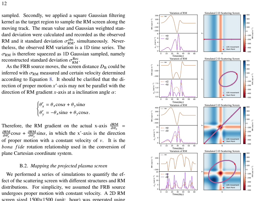
In practice, the proper motion of the FRB source projected on the foreground scattering screen is one-dimensionally sam- pled as a function of angular distance𝜃as it moves. Therefore, the observed RM fluctuation is expected to be1√ 2 smaller than B.DEMONSTRATION VIA SIMULATED FOREGROUND SCREENS The𝐷 S of these three FRBs could be also estimated from simul...
work page 2022
-
[3]
It should be clarified that the di- rection of proper motion𝑥 ′-axis may not be parallel with the direction of RM gradient𝑥-axis at a inclination angle𝛼: ( 𝜃′ 𝑥 =𝜃 𝑥cos𝛼+𝜃 𝑦sin𝛼 𝜃′ 𝑦 =−𝜃 𝑥sin𝛼+𝜃 𝑦cos𝛼. Therefore, the RM gradient on the actual x-axis 𝜕RM 𝜕 𝜃𝑥 = 𝜕RM 𝜕 𝜃′𝑥 cos𝛼+ 𝜕RM 𝜕 𝜃′𝑦 sin𝛼, in which the x’-axis is the direction of proper motion with a co...
work page 2022
-
[4]
with respect to the screen, originated in the lower left. The eccentricity is set to𝑒=0.75 with an inclination angle𝑖=30 ◦ and semi-major axis𝑎=400 (unit: hrs). The orbital elements are selected Under the selected orbital elements, the hypothetical FRB source passes through the red region, in accordance with the fitted binary orbit in F. Y. Wang et al. (2...
work page 2022
-
[5]
C.OBSERV ATIONAL OVERVIEW To provide a simultaneous analysis on propagation effects and its evolution of the selected repeating FRBs, we combined long-term observaions operated by multi-band telescopes.The observational properties of selected bursts are summarized as follows. FRB 20190520B: R. Anna-Thomas et al. (2023) reported the RM variation of FRB 201...
work page 2023
-
[6]
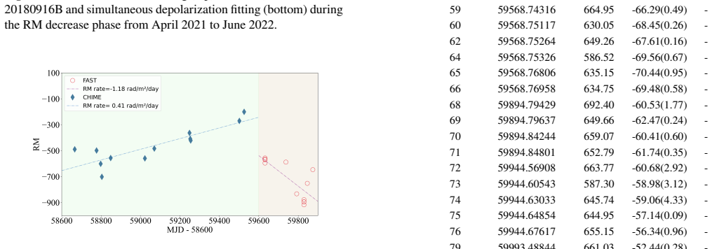
FRB 20180916B: The absolute value of RM was observed to show a nearly linear decrease trend in 2021 across multi- ple telescopes covering from 110 MHz to 5 GHz (Z. Pleunis et al. 2021; R. Mckinven et al. 2023b; S. Bethapudi et al. 2023, 2025), suggesting either a dilution of the electron density or a weakening of the line-of-sight magnetic field component...
work page 2021
-
[7]
or artificial inspection. Figure 7.The variation of scattering (top) and RM (middle) of FRB 201905202B, and simultaneous depolarization fitting (bottom) in three stages. The black dashed lines in the bottom panel represent the fitted depolarization curve by Y. Feng et al. (2022), plotted as reference. The purple shaded regions indicate the 1𝜎uncertainty o...
work page 2022
-
[8]
Later sim- liar scattering timescales were observed by LOFAR during the RM decrease phase (A
when the corresponding RM kept constant. Later sim- liar scattering timescales were observed by LOFAR during the RM decrease phase (A. Gopinath et al. 2024), which implies a relatively stable scattering screen in the local environment of FRB 20180916B. We fitted the linear decrease rate of RM and the simultaneous depolarization of FRB 20180916B. The resul...
work page 2024
-
[9]
CHIME and FAST sequently. The linear fitting of RM vari- ation in two stages turns out to be 0.41 rad/m2/day and -1.18 rad/m2/day, respectively. FRB 20190417A: The RM of FRB 20190417A seemed to fluctuate around 4500 rad/m2 during the FAST observations but remained constant at the same orders of magnitude. The linear changing rate of RM was fitted througho...
-
[10]
Blue diamond and red hollow circles represent the FRBs observed by CHIME and FAST, respectively
Figure 11.The variation of RM of FRB 20190417A. Blue diamond and red hollow circles represent the FRBs observed by CHIME and FAST, respectively. Table 5.Continuous Number MJD Frequency RM L/I - - (MHz) rad/m 2 - 51 59275.47513 587.30 -108.12(0.99) - 52 59275.48829 661.42 -112.77(0.24) - 53 59275.49104 614.36 -116.97(3.71) - 54 59275.51090 680.76 -123.44(4...
-
[11]
and𝑚 p is the mass of the protons. The DM0 contributed by the stellar wind is DMw,0 ≃𝑛 w(𝑎) ·𝑎= ¤𝑀 4𝜋𝑣 w𝜇i𝑚p𝑎2 ·𝑎 ≈5 pc cm −3𝑣 −1 w,8 ¤𝑀 10−8 𝑀⊙yr−1 𝑎 1 AU −1 . (E7) The large-scale magnetic field in the wind is𝐵(𝑟) ∼ 𝐵0 (𝑟/𝑅 ★) −𝛽 , where𝐵 0 is the magnetic field strength. The slope is𝛽=2 for a radial field and𝛽=1 for a toroidal field. The RM0 contribute...
work page 2023
-
[12]
𝜎RM ≃ Δ𝑅 𝑙s 1/2 𝛿RM (𝑙s) ≃2.6 rad m −2 Δ𝑅 10𝑅 ⊙ 1/2 𝑙s 1011 cm −1/2 𝛿RM 1 rad m−2 , (E10) whereΔ𝑅is the thickness of the magnetized plasma screen and𝑙 s ∼10 10 −10 11 cm is the size of clumps in the stellar wind (Z. Y. Zhao et al. 2023). 18 E.2.Supernova remnant Supernova explosion kick velocity of a newborn NS is up to𝑉 k ∼10 3 km/s (S. Park et al. 2012)...
work page 2023
-
[13]
The minimum SNR age is determined by Equation (E11), and the maximum age is taken as the active timescale of the magnetar (𝑡act ∼10 4 yr), so the size of the SNR is∼5−20 pc. E.3.Clumps in SNR The RM variations of FRBs could also be attributed to filaments in SNRs across the line of sight (J. I. Katz 2021). From the X-ray observations of SNRs, the size of ...
work page 2021
discussion (0)
Sign in with ORCID, Apple, or X to comment. Anyone can read and Pith papers without signing in.