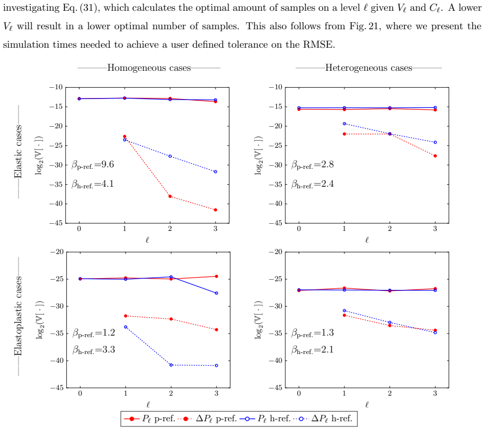
h- and p-refined Multilevel Monte Carlo Methods for Uncertainty Quantification in Structural Engineering
Pith reviewed 2026-05-25 16:51 UTC · model grok-4.3
The pith
Multilevel Monte Carlo and quasi-Monte Carlo with h- and p-refinements deliver significant speedup over standard Monte Carlo for uncertainty quantification in structural beam problems.
A machine-rendered reading of the paper's core claim, the machinery that carries it, and where it could break.
Core claim
By combining h- and p-refinement hierarchies with MLMC and MLQMC, the computational cost for estimating statistics in structural engineering problems with material uncertainty can be reduced significantly compared to standard Monte Carlo sampling, with MLQMC achieving optimal complexity under suitable conditions, p-refinement outperforming h-refinement for random-field models, and the uncertainty representation affecting the resulting solution bounds.
What carries the argument
The multilevel difference estimator across a hierarchy of h- or p-refined meshes that computes solution differences between successive levels to achieve variance reduction while controlling bias.
If this is right
- MLMC and MLQMC achieve significant speedup over MC regardless of whether h- or p-refinement is used.
- MLQMC cost is optimally proportional to 1/epsilon under certain conditions.
- When uncertainty is modeled as a random field, multilevel methods combined with p-refinement have lower computation cost than those based on h-refinement.
- The choice of uncertainty model affects the uncertainty bounds obtained in the solutions.
Where Pith is reading between the lines
- The relative advantage of p-refinement over h-refinement may grow with the number of random variables in the Karhunen-Loève expansion.
- Adaptive selection of refinement type per level could further reduce cost if the correlation structure of the random field varies across scales.
- The observed speedups suggest the approach may transfer to other linear and mildly nonlinear finite-element models beyond the cantilever beam.
Load-bearing premise
The chosen hierarchy of h- and p-refinements produces variance reduction factors that make the multilevel estimators cheaper than standard Monte Carlo for the Gamma and KL-based uncertainty models on the tested beam problems.
What would settle it
Running the same cantilever beam problems and finding that the total wall-clock cost of MLMC or MLQMC exceeds the cost of plain Monte Carlo at the same root-mean-square error tolerance.
Figures


read the original abstract
Practical structural engineering problems are often characterized by significant uncertainties. Historically, one of the prevalent methods to account for this uncertainty has been the standard Monte Carlo (MC) method. Recently, improved sampling methods have been proposed, based on the idea of variance reduction by employing a hierarchy of mesh refinements. We combine an h- and p-refinement hierarchy with the Multilevel Monte Carlo (MLMC) and Multilevel Quasi-Monte Carlo (MLQMC) method. We investigate the applicability of these novel combination methods on three structural engineering problems, for which the uncertainty resides in the Young's modulus: the static response of a cantilever beam with elastic material behavior, its static response with elastoplastic behavior, and its dynamic response with elastic behavior. The uncertainty is either modeled by means of one random variable sampled from a univariate Gamma distribution or with multiple random variables sampled from a gamma random field. This random field results from a truncated Karhunen-Lo\`eve (KL) expansion. In this paper, we compare the computational costs of these Monte Carlo methods. We demonstrate that MQLMC and MLMC have a significant speedup with respect to MC, regardless of the mesh refinement hierarchy used. We empirically demonstrate that the MLQMC cost is optimally proportional to 1/epsilon under certain conditions, where epsilon is the tolerance on the root-mean-square error (RMSE). In addition, we show that, when the uncertainty is modeled as a random field, the multilevel methods combined with p-refinement have a significant lower computation cost than their counterparts based on h-refinement. We also illustrate the effect the uncertainty models have on the uncertainty bounds in the solutions.
Editorial analysis
A structured set of objections, weighed in public.
Referee Report
Summary. The paper proposes combining h- and p-refinement hierarchies with Multilevel Monte Carlo (MLMC) and Multilevel Quasi-Monte Carlo (MLQMC) methods for uncertainty quantification in structural engineering. Numerical experiments are presented on three cantilever beam problems (elastic static, elastoplastic static, elastic dynamic) with Young's modulus uncertainty modeled either by a univariate Gamma random variable or a truncated Karhunen-Loève random field; the central claims are that MLMC and MLQMC deliver significant speedups over standard Monte Carlo regardless of the chosen refinement hierarchy, that MLQMC cost scales optimally as O(1/epsilon) under certain conditions, and that p-refinement yields lower cost than h-refinement when the uncertainty is a random field.
Significance. If the reported empirical speedups and scaling hold under reproducible conditions, the work supplies concrete evidence that multilevel sampling combined with mixed h/p refinement can reduce computational cost for practical engineering UQ problems involving uncertain material properties, extending the applicability of MLMC/MLQMC beyond standard h-refinement hierarchies.
major comments (2)
- [Abstract and numerical experiments] Abstract and numerical experiments section: the headline claim that speedups occur 'regardless of the mesh refinement hierarchy used' is supported only by timing comparisons on three specific beam configurations with Gamma or truncated KL models; without tabulated values of the observed variance decay exponent beta and cost growth exponent gamma for each hierarchy, it is impossible to verify that the reported cost reductions are not particular to the tested meshes, sample counts, and material models.
- [Abstract] Abstract: the statement that 'the MLQMC cost is optimally proportional to 1/epsilon under certain conditions' is presented without accompanying convergence plots, reported beta/gamma pairs, or statistical validation of the RMSE tolerance, leaving the 'certain conditions' qualifier unverified and the scaling claim load-bearing but unsupported by explicit rate analysis.
minor comments (1)
- [Abstract] Abstract: the abbreviation 'MQLMC' appears once and is presumably a typographical variant of MLQMC; consistent terminology should be used throughout.
Simulated Author's Rebuttal
We thank the referee for the constructive comments. We address each major point below and will revise the manuscript accordingly to strengthen the presentation of the empirical results.
read point-by-point responses
-
Referee: [Abstract and numerical experiments] Abstract and numerical experiments section: the headline claim that speedups occur 'regardless of the mesh refinement hierarchy used' is supported only by timing comparisons on three specific beam configurations with Gamma or truncated KL models; without tabulated values of the observed variance decay exponent beta and cost growth exponent gamma for each hierarchy, it is impossible to verify that the reported cost reductions are not particular to the tested meshes, sample counts, and material models.
Authors: We agree that tabulated beta and gamma values per hierarchy would make the verification of the speedup claims more transparent and reproducible. In the revised manuscript we will add a table in the numerical experiments section that reports the observed variance decay exponent beta and cost growth exponent gamma (with standard errors from the fitting procedure) for every combination of refinement hierarchy, uncertainty model, and problem considered. This will directly support the statement that the observed speedups are consistent with the theoretical MLMC/MLQMC complexity bounds across the tested hierarchies. revision: yes
-
Referee: [Abstract] Abstract: the statement that 'the MLQMC cost is optimally proportional to 1/epsilon under certain conditions' is presented without accompanying convergence plots, reported beta/gamma pairs, or statistical validation of the RMSE tolerance, leaving the 'certain conditions' qualifier unverified and the scaling claim load-bearing but unsupported by explicit rate analysis.
Authors: We accept that the abstract claim requires explicit supporting material. The revised version will include (i) convergence plots of computational cost versus RMSE tolerance for the MLQMC runs that exhibit the optimal O(1/epsilon) scaling, (ii) the corresponding beta/gamma pairs already planned for the new table, and (iii) a short clarification in both the abstract and the numerical section that identifies the precise hierarchies and random-field models for which the optimal scaling is observed. These additions will remove any ambiguity about the 'certain conditions'. revision: yes
Circularity Check
No significant circularity: claims are direct empirical observations on specific test cases
full rationale
The paper's central claims consist of measured speedups and observed cost scaling O(1/epsilon) obtained by running MC, MLMC and MLQMC on three concrete cantilever-beam problems (elastic static, elastoplastic static, elastic dynamic) with either univariate Gamma or truncated KL random fields. These outcomes are reported as numerical results for the chosen hierarchies and sample counts; no parameters are fitted to a subset of data and then invoked as predictions of related quantities, no self-definitional equations appear, and no load-bearing uniqueness theorems or ansatzes are imported via self-citation. The derivation chain is therefore self-contained against external benchmarks and receives the default non-circularity finding.
Axiom & Free-Parameter Ledger
free parameters (1)
- Hierarchy levels and KL truncation order
axioms (1)
- domain assumption Gamma distribution or truncated KL expansion of a gamma random field adequately represents spatial uncertainty in Young's modulus for the beam problems.
Reference graph
Works this paper leans on
-
[1]
M. Kleiber, T. D. Hien, The stochastic finite element method basic perturbation technique and computer implementation, Wiley, U.K., 1992
work page 1992
-
[2]
R. G. Ghanem, P. D. Spanos, Stochastic Finite Elements: A Spectral Approach, Dover Publications, New York, 2003
work page 2003
-
[3]
I. Babuka, F. Nobile, R. Tempone, A stochastic collocation method for elliptic partial differential equations with random input data, SIAM J. Numer. Anal. 45 (3) (2007) 1005–1034. doi:10.1137/050645142
-
[4]
G. S. Fishman, Monte Carlo: concepts, algorithms and applications, Springer-Verlag, New York, 1996
work page 1996
-
[5]
R. E. Caflisch, Monte Carlo and Quasi-Monte Carlo methods, Acta Numerica 7 (1998) 1–49. doi:10.1017/ S0962492900002804
work page 1998
-
[6]
Niederreiter, Monte Carlo and Quasi-Monte Carlo methods, Springer, Berlin, 2004
H. Niederreiter, Monte Carlo and Quasi-Monte Carlo methods, Springer, Berlin, 2004
work page 2004
-
[7]
Loh, On latin hypercube sampling, Ann
W.-L. Loh, On latin hypercube sampling, Ann. Statist. 24 (5) (1996) 2058–2080. doi:10.1214/aos/1069362310
-
[8]
M. B. Giles, Multilevel Monte Carlo path simulation, Operations Research 56 (3) (2008) 607–617. doi:10.1287/opre. 1070.0496. 31
-
[9]
M. B. Giles, B. J. Waterhouse, Multilevel Quasi-Monte Carlo path simulation, Radon Series on Computational and Applied Mathematics 8 (2009) 1–18
work page 2009
-
[10]
P. Robbe, D. Nuyens, S. Vandewalle, A Multi-Index Quasi-Monte Carlo algorithm for lognormal diffusion problems, SIAM J. Sci. Comput. 39 (5) (2017) S851–S872. doi:10.1137/16M1082561
- [11]
-
[12]
Ghanem, Hybrid stochastic finite elements and generalized Monte Carlo simulation, J
R. Ghanem, Hybrid stochastic finite elements and generalized Monte Carlo simulation, J. Appl. Mech. 65 (4) (1998) 1004–1009. doi:10.1115/1.2791894
-
[13]
S. Acharjee, N. Zabaras, A non-intrusive stochastic galerkin approach for modeling uncertainty propagation in deformation processes, Comput. Struct. 85 (5) (2007) 244–254. doi:10.1016/j.compstruc.2006.10.004
-
[14]
Shinozuka, Monte Carlo solution of structural dynamics, Comput
M. Shinozuka, Monte Carlo solution of structural dynamics, Comput. Struct. 2 (5) (1972) 855–874. doi:10.1016/ 0045-7949(72)90043-0
work page 1972
-
[15]
J. Pulido, T. Jacobs, E. de Lima, Structural reliability using Monte Carlo simulation with variance reduction techniques on elastic-plastic structures, Comput. Struct. 43 (3) (1992) 419–430. doi:10.1016/0045-7949(92)90275-5
-
[16]
Y. Liu, M. D. Shields, A direct simulation method and lower-bound estimation for a class of gamma random fields with applications in modelling material properties, Probab. Eng. Mech. 47 (2017) 16–25. doi:10.1016/j.probengmech.2017. 01.001
-
[17]
E. Simoen, B. Moaveni, J. P. Conte, G. Lombaert, Uncertainty quantification in the assessment of progressive damage in a 7-story full-scale building slice, J. Eng. Mech. 139 (12) (2013) 1818–1830. doi:10.1061/(ASCE)EM.1943-7889.0000610
-
[18]
P. E. Hess, D. Bruchman, I. A. Assakkaf, B. M. Ayyub, Uncertainties in material and geometric strength and load variables, Naval Engineers Journal 114 (2) (2002) 139–166. doi:10.1111/j.1559-3584.2002.tb00128.x
-
[19]
Lo` eve, Probability theory, Springer, New York, 1977
M. Lo` eve, Probability theory, Springer, New York, 1977
work page 1977
-
[20]
Grigoriu, Simulation of stationary non-gaussian translation processes, J
M. Grigoriu, Simulation of stationary non-gaussian translation processes, J. Engrg. Mech. (ASCE) 124 (2) (1998) 121–126. doi:10.1061/(ASCE)0733-9399(1998)124:2(121)
-
[21]
K. Atkinson, W. Han, Numerical Solution of Fredholm Integral Equations of the Second Kind, Springer New York, New York, NY, 2009, pp. 473–549. doi:10.1007/978-1-4419-0458-4_12
-
[22]
R. de Borst, M. A. Crisfield, J. J. C. Remmers, NonLinear Finite Element Analysis of Solids and Structures, Wiley, U.K., 2012
work page 2012
-
[23]
A. Prez-Foguet, A. Rodrguez-Ferran, A. Huerta, Consistent tangent matrices for substepping schemes, Comput.Methods in Appl.Mech.Eng 190 (35) (2001) 4627–4647. doi:10.1016/S0045-7825(00)00336-4
-
[24]
M. B. Giles, Multilevel Monte Carlo methods, Acta Numerica 24 (2015) 259–328. doi:10.1017/S096249291500001X
-
[25]
J. Dick, F. Y. Kuo, I. H. Sloan, High-dimensional integration: The Quasi-Monte Carlo way, Acta Numerica 22 (2013) 133–288. doi:10.1017/S0962492913000044
-
[26]
F. Y. Kuo, R. Scheichl, C. Schwab, I. H. Sloan, E. Ullmann, Multilevel Quasi-Monte Carlo methods for lognormal diffusion problems, Math. Comput. 86 (308) (2017) 2827–2860. doi:10.1090/mcom/3207
-
[27]
F. Y. Kuo, D. Nuyens, Application of Quasi-Monte Carlo methods to elliptic pdes with random diffusion coefficients: A survey of analysis and implementation, Foundations of Computational Mathematics 16 (6) (2016) 1631–1696. doi: 10.1007/s10208-016-9329-5
-
[28]
I. H. Sloan, H. Woniakowski, When are Quasi-Monte Carlo algorithms efficient for high dimensional integrals?, J. Com- plexity 14 (1) (1998) 1–33. doi:10.1006/jcom.1997.0463
-
[29]
A. L. Teckentrup, Multilevel Monte Carlo methods and uncertainty quantification, Ph.D. thesis, University of Bath, http://www.maths.bath.ac.uk/~masrs/Teckentrup_PhD.pdf (2013). 32
work page 2013
-
[30]
D. Drzisga, B. Gmeiner, U. Rde, R. Scheichl, B. Wohlmuth, Scheduling massively parallel multigrid for Multilevel Monte Carlo methods, SIAM Journal on Scientific Computing 39 (5) (2017) S873–S897. doi:10.1137/16M1083591
-
[31]
J. Li, J. Chen, Stochastic Dynamics of Structures, Wiley, Asia, 2010
work page 2010
-
[32]
C. E. Brenner, C. Bucher, A contribution to the sfe-based reliability assessment of nonlinear structures under dynamic loading, Probab. Eng. Mech. 10 (4) (1995) 265 – 273. doi:10.1016/0266-8920(95)00021-6. 33
discussion (0)
Sign in with ORCID, Apple, or X to comment. Anyone can read and Pith papers without signing in.