REVIEW 2 major objections 4 minor 23 references
An Adaptive Pole-Matching Method for Interpolating Reduced-Order Models
T0 review · 2 major / 4 minor · reviewed 2026-08-14 · deepseek-v4-flash
Pith's one-line read Pole matching makes reduced parametric models 100x more accurate
desk verdict Useful adaptive PMOR framework, but the 'branch-and-bound' pole matcher is really a 2-opt heuristic, so the global optimality claim doesn't hold up. read the letter →
The pith
A machine-rendered reading of the paper's core claim, the machinery that carries it, and where it could break.
The reading
What carries the argument
The central object is the pole-residue realization of a reduced-order model: every pole (real or conjugate-complex pair) is stored with its residue, so a ROM is represented by a small matrix of pole positions and residue weights. The argument runs through the pole-matching optimization, which minimizes a weighted Frobenius distance between pole-residue matrices over row permutations, decoupled into independent problems for complex and real poles; the branch-and-bound algorithm (Algorithm III.1) uses the swap-pruning Theorem III.1 to avoid exhaustive enumeration. The adaptive framework then rides on two mechanisms: a predictor-corrector rule that chooses the reference ROM for matching, and a midpoint error check comparing an interpolated ROM against a freshly computed ROM that triggers refinement. Regression is the compression mechanism that stores polynomial coefficients instead of the full repository.
What would settle it
Construct two small ROMs whose correct pole matching is known by construction to require two swaps, with the first swap increasing the weighted distance; run Algorithm III.1 from the natural ordering. If it returns the wrong permutation, the central matching guarantee fails. A practical version is to take a diagonal parameterized system with two pairs of poles whose dominance crosses, build ROMs at two parameter values, compute the known optimal matching by exhaustive search, and compare it with the branch-and-bound result.
Extended reading notes
Core claim
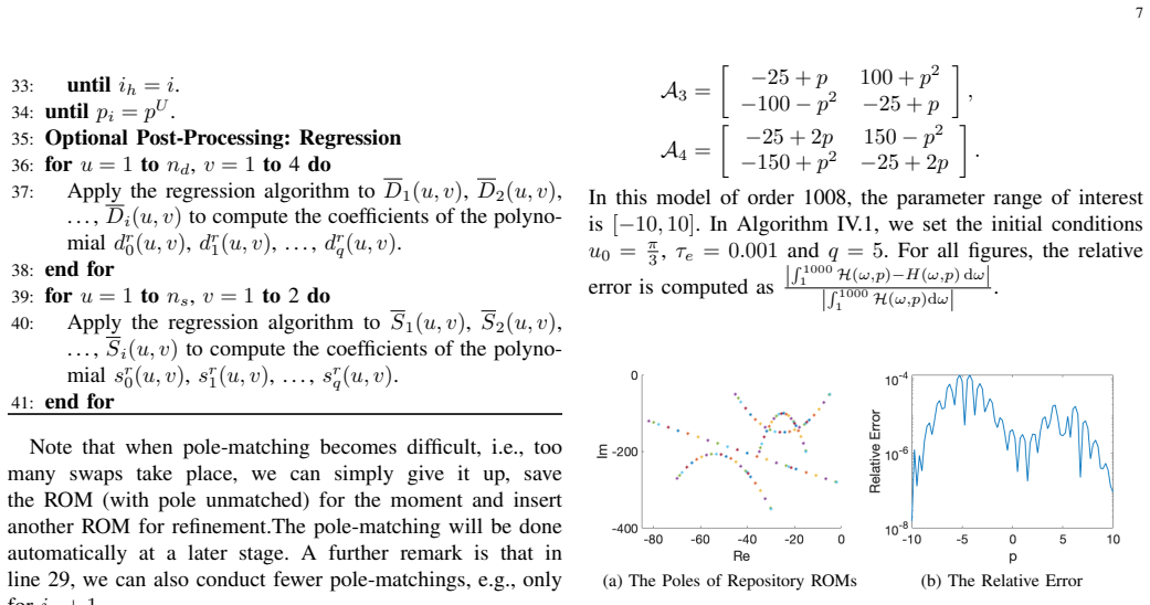
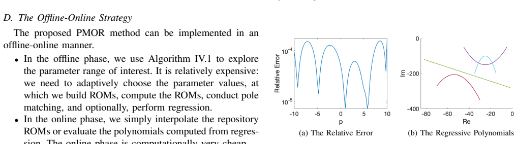
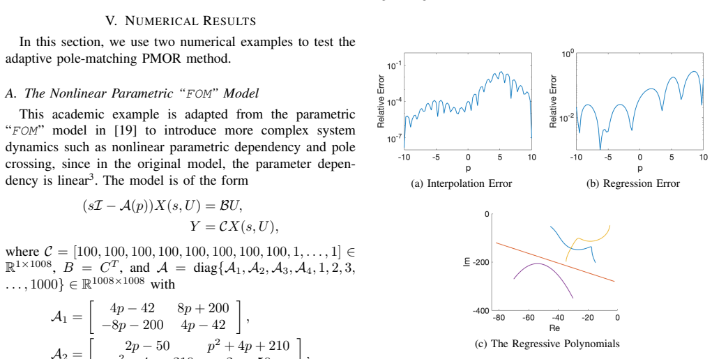
The paper's claim is that pole-residue data are the right quantities to interpolate when building a parametric reduced-order model, provided the poles are first matched correctly and the repository ROMs are placed adaptively. All local ROMs are transformed into a pole-residue realization, where the transfer function is a sum of terms each determined by a pole position and a residue; the paper then treats matching as a weighted least-squares assignment of rows between two ROMs and solves it with a branch-and-bound search whose pruning rule is supplied by Theorem III.1. Because matching is reliable only for perturbed poles, the framework uses a predictor-corrector strategy: a predicted ROM is extrapolated from already-built repository ROMs and used as the reference for matching the candidate ROM, and an adaptive refinement loop inserts an extra ROM at the midpoint whenever the interpolated ROM fails an error check against a freshly computed ROM. An optional regression phase replaces the stored repository by entrywise polynomials in the parameter. The numerical experiments report that the full framework reduces relative error from the $10^{-2}$ magnitude to $10^{-4}$ and reduces storage relative to the interpolated repository.
Load-bearing premise
The load-bearing premise is that the branch-and-bound search, which only tries single swaps and stops when no swap lowers the matching cost, returns the correct pole correspondence; if the true correspondence requires a sequence of swaps where some intermediate swap looks worse, the matching can be wrong and the interpolation corrupted.
Editorial extensions
If this is right
- Any model-order reduction method can feed the framework, since only accurate local ROMs are required and the state-space form of the full-order model is never needed globally.
- The pROM size stays constant as the number of parameters grows, because only pole and residue entries are stored and interpolated, not a global projection subspace.
- Complicated parameter dependence, including pole crossing, can be captured locally by adaptive step selection without assuming affine parameter dependence.
- Storage can be cut from $N(4n_d+2n_s)$ repository entries to $(q+1)(4n_d+2n_s)$ polynomial coefficients when the regression post-processing is used.
- Stability is easy to monitor because the interpolated model is built directly from pole positions; linear interpolation in the left half-plane preserves stability.
Reading between the lines
- A robust global solver for the pole-matching assignment, rather than a local swap search, would let the same framework interpolate ROMs whose pole orderings differ strongly, extending it to heterogeneous ROM sources in industrial practice.
- The midpoint error check could be developed into an a posteriori error estimator: if the interpolated-ROM error correlates with the distance between neighboring repository parameters, the same loop could certify accuracy over the whole parameter interval.
- For non-normal systems, where small parameter changes can move poles abruptly, a natural extension is to match pseudospectral regions or dominant invariant subspaces instead of individual poles; the paper itself notes pole sensitivity as a limitation.
Signed reviews
Editorial analysis
A structured set of objections, weighed in public.
Referee Report
Summary. The paper proposes an adaptive parametric reduced-order modeling (PMOR) method based on interpolating the poles and residues of local reduced-order models (ROMs). Pole matching between ROMs at nearby parameter values is formulated as a combinatorial optimization problem, which the authors claim to solve with a branch-and-bound algorithm (Section III-B). The adaptive framework (Algorithm IV.1) combines a predictor-corrector strategy, an adaptive refinement strategy using a test-ROM at interval midpoints, and an optional polynomial-regression post-processing step. Numerical experiments on an academic 1008-state example and a branchline-coupler microwave model report relative errors around 10^-4 and reduced storage.
Significance. If the central claims hold, the method would be a useful contribution: it is compatible with any MOR method, uses a pole-residue realization that removes coordinate-system ambiguity, and the adaptive refinement loop validates interpolated ROMs against freshly computed ROMs, which is an external and non-circular check. The numerical results are encouraging and the storage reduction via regression is clearly demonstrated. However, the correctness of the entire framework rests on the pole-matching optimization, and the paper does not establish that Algorithm III.1 solves that optimization globally. The two examples are also limited to a single parameter, so the broader advantages stated in the abstract are not yet demonstrated.
major comments (2)
- [Section III-B, Theorem III.1 and Algorithm III.1] Algorithm III.1 is presented as a branch-and-bound solver for the global optimization problem (14), but it is actually a greedy local search: it starts from the identity permutation, accepts a new permutation only when a single transposition strictly decreases the objective, and terminates when no allowed transposition improves it. The objective in (14) decomposes as a sum of independent row costs and is a linear assignment problem. For such problems, a permutation that is locally optimal under all single transpositions need not be globally optimal; a 3-cycle can have strictly lower cost than the identity even when every transposition increases the cost. Theorem III.1 only proves that the specific swapped configuration tested is not optimal, and it gives no bound that would rule out such cycles. Therefore the statement that Algorithm III.1 'solves' (14) or 'guarantees correct pole-matching' is unsupported. This is load-bearing: Section VI and Fig. 3 show that a wrong matching can globally corrupt the regression, and the adaptive refinement strategy does not cure this when mismatched poles have similar positions and residues.
- [Section III-B, F-matrix update rule (lines 10-11 and Eq. (22))] The pruning bookkeeping with the matrix F does not follow from Theorem III.1. In the theorem, a failed swap of the i-th and j-th entries at the current permutation vd forbids any assignment with vd_i = B and vd_j = A, where A = vd_i and B = vd_j before the swap. The update F(vd_i, vd_j) = 0, however, forbids the condition vd_{vd_i} = vd_j and vd_{vd_j} = vd_i, which is a different condition unless the current permutation happens to satisfy vd_i = i and vd_j = j. Consequently, the algorithm may prune permutations that Theorem III.1 does not rule out, or fail to prune permutations that it does rule out. This undermines the claimed branch-and-bound efficiency and correctness even for a single swap.
minor comments (4)
- [Introduction, Section I] The phrase 'brutal-force method' should be 'brute-force method'.
- [Section V, relative error definition] In the definition of the relative error, the integrand in the numerator appears as H(ω,p) minus H(ω,p), which is identically zero; presumably the second factor should be the pROM transfer function, e.g., \hat H(ω,p).
- [References [14] and [15]] The conference title is given as 'Numerical Electromagnetic and Metaphysics Modeling and Optimization'; it should be 'Numerical Electromagnetic and Multiphysics Modeling and Optimization'.
- [Section IV-C and abstract] The paper confines the adaptive framework to a single scalar parameter (Section IV), yet the abstract claims 'constant size of the parametric reduced-order model with respect to the number of parameters' and 'capability to deal with complicated parameter dependency'; these broader claims are not supported by the numerical results in this manuscript.
Circularity Check
No significant circularity: the derivation is self-contained and the accuracy claims are checked against freshly computed ROMs and the true FOM, not against fitted inputs.
full rationale
The paper's derivation chain is not circular. The pole-matching objective in (13)-(15) is an optimization over row permutations with user-chosen weighting matrices; it is not fitted to any quantity that is later reported as a prediction. The local ROMs are computed by standard MOR algorithms, and the pole-residue realization in Section II is fully restated in the paper rather than imported as an unverified self-citation. The adaptive refinement strategy in Algorithm IV.1 validates each interval by comparing an interpolated ROM_I,t against a freshly built ROM_T,t at the midpoint (line 20, criterion (28)); ROM_T,t is generated independently by a MOR algorithm, so the acceptance test is an external benchmark. The optional regression post-processing fits polynomials to the repository ROM entries and is then evaluated against the true full-order model in Section V, again an external comparison. The self-citations [9], [14], [15] provide background and prior contributions, but the new claims—branch-and-bound pole-matching, predictor-corrector, adaptive refinement—are not derived from those citations. The main weakness, that Algorithm III.1 is a local swap search and Theorem III.1 only proves a pruning rule rather than global optimality for (14), is a correctness risk and not a circularity; it does not make the validation self-referential.
Assumptions & free parameters
free parameters (4)
- wp, wr (pole position/residue weights)
- τe (error tolerance) =
0.001 (Example 1), 0.00001 (Example 2)
- u0 (initial step length) =
π/3 (Example 1)
- q (regression polynomial degree) =
5 (Example 1), 7 (Example 2)
assumptions (4)
- domain assumption Assumption III.1: The sizes of D and S in the two ROMs are equal and the poles of ROM2 are perturbations of ROM1.
- domain assumption Assumption IV.1: A high-accuracy ROM can be built at any feasible parameter value on request.
- domain assumption Assumption IV.2: Pole positions and residues change smoothly with the parameter p for small parameter changes.
- domain assumption Assumption III.2: The identity permutation is a good initial guess when the same MOR method preserves eigenvalue order under small parameter perturbations.
Cite this review
Pith. "Pith review of An Adaptive Pole-Matching Method for Interpolating Reduced-Order Models." pith.science (2026). https://pith.science/paper/RCVBVDY6
@misc{pith2026190800820,
  author       = {Pith},
  title        = {Pith review of: An Adaptive Pole-Matching Method for Interpolating Reduced-Order Models},
  year         = {2026},
  howpublished = {\url{https://pith.science/paper/RCVBVDY6}},
  note         = {Machine review of arXiv:1908.00820}
}
read the original abstract
An adaptive parametric reduced-order modeling method based on interpolating poles of reduced-order models is proposed in this paper. To guarantee correct interpolation, a pole-matching process is conducted to determine which poles of two reduced-order models correspond to the same parametric pole. First, the pole-matching in the scenario of parameter perturbation is discussed. It is formulated as a combinatorial optimization problem and solved by a branch and bound algorithm. Then, an adaptive framework is proposed to build repository ROMs at adaptively chosen parameter values, which well represent the parameter domain of interest. To achieve this, we propose techniques including a predictor-corrector strategy and an adaptive refinement strategy, which enable us to use larger steps to explore the parameter domain of interest with good accuracy. The framework also consists of regression as an optional post-processing phase to further reduce the data storage. The advantages over other parametric reduced-order modeling approaches are, e.g., compatibility with any model order reduction method, constant size of the parametric reduced-order model with respect to the number of parameters, and capability to deal with complicated parameter dependency.
Figures
Figures from the paper (1 more)

Reference graph
Works this paper leans on
-
[1]
A survey of model reduction methods for parametric systems,
P. Benner, S. Gugercin, and K. Willcox, “A survey of model reduction methods for parametric systems,” SIAM Review, vol. 57, no. 4, pp. 483– 531, 2015
work page 2015
-
[2]
L. Feng, Y . Yue, N. Banagaaya, P. Meuris, W. Schoenmaker, and P. Benner, “Parametric modeling and model order reduction for (electro-)thermal analysis of nanoelectronic structures,” J. Math. Ind. , vol. 6, no. 1, pp. 1–10, 2016
work page 2016
-
[3]
Y . Yue and K. Meerbergen, “Using Krylov-Pad ´e model order reduction for accelerating design optimization of structures and vibrations in the frequency domain,” International Journal for Numerical Methods in Engineering, vol. 90, no. 10, pp. 1207–1232, 2012
work page 2012
-
[4]
Parametric dominant pole algorithm for parametric model order reduction,
M. Saadvandi, K. Meerbergen, and W. Desmet, “Parametric dominant pole algorithm for parametric model order reduction,” Journal of Com- putational and Applied Mathematics , vol. 259, pp. 259–280, 2014
work page 2014
-
[5]
Y . Zhang, L. Feng, S. Li, and P. Benner, “Accelerating PDE constrained optimization by the reduced basis method: application to batch chro- matography,” Internat. J. Numer. Methods Engrg. , vol. 104, no. 11, pp. 983–1007, 2015
work page 2015
-
[6]
G. Rozza, D. B. P. Huynh, and A. T. Patera, “Reduced basis approxima- tion and a posteriori error estimation for affinely parametrized elliptic coercive partial differential equations,”Archives of Computational Meth- ods in Engineering , vol. 15, no. 3, pp. 229–275, 2008
work page 2008
-
[7]
Interpolatory projection methods for parameterized model reduction,
U. Baur, C. A. Beattie, P. Benner, and S. Gugercin, “Interpolatory projection methods for parameterized model reduction,” SIAM J. Sci. Comput., vol. 33, no. 5, pp. 2489–2518, 2011
work page 2011
-
[8]
D. Amsallem and C. Farhat, “Interpolation method for the adaptation of reduced-order models to parameter changes and its application to aeroelasticity,” AIAA J., vol. 46, pp. 1803–1813, 2008
work page 2008
Show all 23 references
-
[9]
Reduced-order modelling of paramet- ric systems via interpolation of heterogeneous surrogates,
Y . Yue, L. Feng, and P. Benner, “Reduced-order modelling of paramet- ric systems via interpolation of heterogeneous surrogates,” Advanced Modeling and Simulation in Engineering Sciences , pp. 1–28, 2019, to appear
2019
-
[10]
Parametric model order reduction by matrix interpolation,
H. Panzer, J. Mohring, R. Eid, and B. Lohmann, “Parametric model order reduction by matrix interpolation,” at-Automatisierungstechnik, vol. 58, no. 8, pp. 475–484, 2010
2010
-
[11]
An online method for interpolating linear parametric reduced-order models,
D. Amsallem and C. Farhat, “An online method for interpolating linear parametric reduced-order models,” SIAM J. Sci. Comput., vol. 33, no. 5, pp. 2169–2198, 2011
2011
-
[12]
Modellreduktion f ¨ur parametrisierte Systeme durch balanciertes Abschneiden und Interpolation (Model Reduction for Parametric Systems Using Balanced Truncation and Interpolation),
U. Baur and P. Benner, “Modellreduktion f ¨ur parametrisierte Systeme durch balanciertes Abschneiden und Interpolation (Model Reduction for Parametric Systems Using Balanced Truncation and Interpolation),” at- Automatisierungstechnik, vol. 57, no. 8, pp. 411–420, 2009
2009
-
[13]
Parameter preserving model reduction for MEMS applications,
U. Baur, P. Benner, A. Greiner, J. G. Korvink, J. Lienemann, and C. Moosmann, “Parameter preserving model reduction for MEMS applications,” Math. Comput. Model. Dyn. Syst. , vol. 17, no. 4, pp. 297– 317, 2011
2011
-
[14]
Interpolation of reduced-order models based on modal analysis,
Y . Yue, L. Feng, and P. Benner, “Interpolation of reduced-order models based on modal analysis,” in2018 IEEE MTT-S International Conference on Numerical Electromagnetic and Metaphysics Modeling and Opti- mization (NEMO), 2018
2018
-
[15]
An adaptive method for interpolating reduced-order models based on matching and continuation of poles,
——, “An adaptive method for interpolating reduced-order models based on matching and continuation of poles,” in 2019 IEEE MTT-S Inter- national Conference on Numerical Electromagnetic and Metaphysics Modeling and Optimization (NEMO) , 2019
2019
-
[16]
G. H. Golub and C. F. van Van Loan, Matrix Computations , 3rd ed. Baltimore and London: The Johns Hopkins University Press, 1996
1996
-
[17]
Branch and bound algorithms — principles and examples,
J. Clausen, “Branch and bound algorithms — principles and examples,” University of Copenhagen, Tech. Rep., 1999
1999
-
[18]
Computing dominant poles of power system transfer functions,
N. Martins, L. T. G. Lima, and H. J. C. P. Pinto, “Computing dominant poles of power system transfer functions,” IEEE Trans. Power Syst. , vol. 11, no. 1, pp. 162–170, 1996
1996
-
[19]
Data-driven parametrized model reduction in the Loewner framework,
A. C. Ionita and A. C. Antoulas, “Data-driven parametrized model reduction in the Loewner framework,” SIAM J. Sci. Comput. , vol. 36, no. 3, pp. A984–A1007, 2014
2014
-
[20]
A collection of benchmark exam- ples for model reduction of linear time invariant dynamical systems,
Y . Chahlaoui and P. Van Dooren, “A collection of benchmark exam- ples for model reduction of linear time invariant dynamical systems,” SLICOT Working Note, Tech. Rep. 2002–2, 2002, available from www.slicot.org
2002
-
[21]
Branchline coupler,
The MORwiki Community, “Branchline coupler,” MORwiki – Model Order Reduction Wiki, 2013. [Online]. Available: http: //modelreduction.org/index.php/Branchline Coupler
2013
-
[22]
Fast evaluation of time-harmonic Maxwell’s equations using the reduced basis method,
M. W. Hess and P. Benner, “Fast evaluation of time-harmonic Maxwell’s equations using the reduced basis method,” IEEE Trans. Microw. Theory Techn., vol. 61, no. 6, pp. 2265–2274, 2013
2013
-
[23]
A. C. Antoulas, Approximation of Large-Scale Dynamical Systems , ser. Advances in Design and Control. Philadelphia, PA: SIAM Publications, 2005, vol. 6
2005
Reviewed August 14, 2026 · model on record in the stance chip above.
Discussion (0). Continue with ORCID to comment.