Functional Ratings in Sports

Abigail Slater; Bradley Lowery; Kaison Thies

REVIEW 4 major objections 6 minor 10 references

Functional Ratings in Sports

T0 review · 4 major / 6 minor · reviewed 2026-08-14 · deepseek-v4-flash

Challenge this review Re-run · record.json Download PDF Read on arXiv ↗ Review JSON

Pith's one-line read Team strength as a curve, not a number: least squares fit to every second of game data yields ratings that predict point differential at any moment.

desk verdict Competent pointwise extension of least-squares ratings to functional data; the descriptive model works, but the predictive claims and inference need more support. read the letter →

arxiv 1908.00939 v1 pith:ZWV3IGTT submitted 2019-08-02 stat.AP

Bradley Lowery , Abigail Slater , Kaison Thies This is my paper · ORCID

classification stat.AP MSC 62J0562P99

keywords functionaldataanalysisleastsquaressportsrankingshome-courtadvantagepointdifferentialbasketballstrengthofscheduletime-varyingratings

verification ladder T0 review T1 audit T2 compute T3 formal

The pith

A machine-rendered reading of the paper's core claim, the machinery that carries it, and where it could break.

The reading

This paper proposes a new way to rank sports teams: instead of using only final scores, it fits a least-squares model at every second of game time, producing a rating curve for each team. The central claim is that the difference of two teams' rating curves equals the expected point differential between them at that time, adjusted for strength of schedule. Using 2018-2019 NCAA men's basketball play-by-play data, the paper argues that a single common home-court advantage curve is the right specification: home advantage is statistically important but does not differ across teams. If correct, the method turns every scoring event into information about team strength and allows prediction of the expected score gap at any moment.

What carries the argument

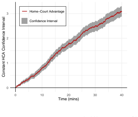
The load-bearing object is the design matrix $X$ together with the pointwise least-squares solution at each second. $X$ encodes each game as a row with $+1$ for the home team, $-1$ for the away team, and $0$ otherwise, and the constraint that the average rating is the zero function fixes the null space. The normal equation $X^\top X\beta(t) = X^\top d(t)$ splits every rating into average point differential and strength of schedule. Model selection uses F-tests at every time point, producing a curve of $P$-values that shows when the constant home-court model is appropriate.

What would settle it

Re-run the analysis after removing the documented data errors—such as the game with only box-score points, missing final scoring plays appended at the final timestamp, and intervals where simultaneous scoring plays are treated as a persistent lead—and check whether the functional ratings and the model-selection P-values change substantially. If they do, the central claim that the ratings reflect true time-varying performance is undermined; if they barely change, the claim is supported.

Watch

Extended reading notes

Core claim

The paper's central discovery is that the pointwise least-squares solution of $X\beta(t) = d(t)$ with the constraint $\sum_i \beta_i(t) = 0$ yields a functional rating $\beta_i(t)$ for each team such that $\beta_i(t) - \beta_j(t)$ is the expected point differential at time $t$ in a neutral-court game between teams $i$ and $j$. The rating naturally decomposes into the team's average point differential plus a time-varying strength-of-schedule component. Comparing three nested models with ANOVA at every second shows that the model with a constant home-court advantage $\alpha(t)$ is needed, while a model with individual team home-court advantages is not, so the constant-home-advantage model is selected for the rest of the analysis.

Load-bearing premise

That the play-by-play scoring data, after interpolation to every second, accurately represents the true score differential at every time, so the pointwise least-squares ratings do not inherit bias from missing or simultaneous scoring plays.

Editorial extensions

If this is right

Team rankings can be computed as weighted averages of the functional ratings, allowing users to favor early-game or late-game performance according to a chosen weight function.
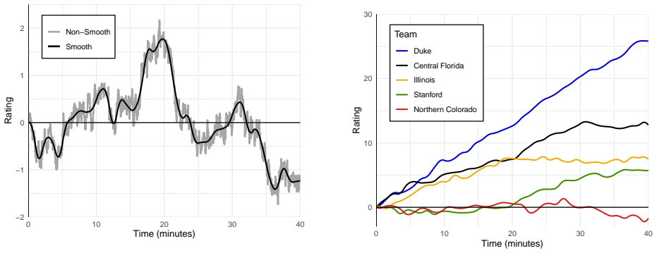
The rating curve reveals a team's playing style, such as being a strong first-half or second-half team, as illustrated by Stanford improving late and Illinois leveling off.
Expected point differential can be predicted between any two teams at any time, even if they never played, and the home-court advantage adds about three points at the end of a game.
The framework extends naturally to other sports with scoring data, though further study is needed to simulate realistic game flows.

Reading between the lines

Editorial extensions of the paper, not claims the author makes directly.

The paper's P-value threshold is informal; a formal functional hypothesis test for the home-court advantage curves could sharpen the model choice and might alter the conclusion if early-game P-values were treated differently.
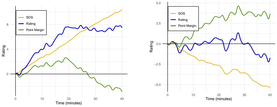
The decomposition $\beta_i(t) = \bar{d}_i(t) + \mathrm{sos}_i(t)$ suggests a time-varying strength-of-schedule measure that could be compared with static strength-of-schedule rankings, potentially offering new insight into schedule difficulty.
Because the documented data errors (missing scoring plays, simultaneous plays treated as persistent leads) could bias specific intervals, a sensitivity analysis that drops or re-times those plays would test whether the ratings and model selection survive the noise.

Share X Bluesky LinkedIn Reddit HN

Signed reviews

No signed human review yet.

Editorial analysis

A structured set of objections, weighed in public.

Desk editor's note, referee report, and a circularity audit.

Desk Editor's Note

read the letter

Colleague,

The thing to know: this is a competent and clearly written extension of scalar least-squares sports ratings to a function-valued rating over game time. The pointwise least-squares algebra is correct, and the schedule-strength decomposition from the normal equations is a nice descriptive payoff. But the paper oversells the word 'prediction': the predictions in Section 5.3 are in-sample fitted differences, and the data errors documented in Section 3.1 are never tested for sensitivity.

What's new: previous least-squares ratings (Stefani, Harville) used final scores; this runs the same regression at each second, producing rating curves. Because there is no temporal coupling, it is a pointwise collection of scalar ratings, not a new estimation principle. Still, the functional view gives a useful way to see when teams are strong and to break a rating into average margin and schedule strength. The authors are transparent about their data problems and about the fact that their 'predicted' game flow is not realistic.

Soft spots, in proportion. The central descriptive model holds up. The bigger issues: first, the model-comparison ANOVA is run at every second without any adjustment for multiple comparisons or temporal correlation; the p-value functions in Figures 1 and 2 are highly correlated, so 'consistently less than .1' is not a formal inference. Second, the data errors are potentially load-bearing. The North Alabama/Samford example shows a 5-point lead assigned to a 213-second interval; if such intervals are common, the pointwise ratings and the home-court conclusion inherit those biases. The paper gives no count of affected games or seconds and no sensitivity analysis. This is fixable but not ignorable. Third, no code or data is provided, so the empirical claims cannot be checked.

Who this is for: sports-analytics readers and functional-data-analysis folks looking for a simple, honest application. It deserves a serious referee, not a desk reject: the method is sound as a descriptive tool, and the deficiencies are addressable. I'd ask the authors for an out-of-sample or cross-validation check, a multiple-comparisons or time-series-aware treatment of the p-value functions, and sensitivity analysis around the data-cleaning choices. With those, the paper would be a reasonable contribution to an applied statistics or sports analytics venue.

Referee Report

4 major / 6 minor

Summary. The paper proposes a functional rating model for sports teams. Given play-by-play score differences d(t) for m games, team ratings β_i(t) are estimated by solving Xβ(t)=d(t) in least squares at each second, with the identifiability constraint Σβ_i(t)=0. Three specifications are considered: no home-court advantage (Model 1), a common home-court advantage α(t) (Model 2), and team-specific advantages α_i(t) (Model 3). The model is applied to 5,603 NCAA Division 1 men's basketball games from the 2018–2019 season. Model selection is performed by computing ANOVA p-values pointwise in time, leading to the choice of Model 2. Ratings are smoothed with fourth-order B-splines, converted to scalar rankings by weighted integrals, and decomposed into average point differential and strength of schedule via the normal equations. The paper also illustrates in-sample 'predictions' of the expected point differential curve for a Duke–Virginia matchup.

Significance. The methodological idea is attractive, and the least-squares algebra is straightforward and largely self-contained. The strength-of-schedule decomposition in Section 5.2 is a nice consequence of the normal equations, and the explicit treatment of identifiability via the sum-to-zero constraint is sound. The paper also deserves credit for candidly documenting the three data-quality problems in Section 3.1. If the empirical claims were supported by out-of-sample validation and sensitivity analysis, the functional rating approach would be a useful addition to sports analytics, going beyond final-score ratings by making the entire time course of performance comparable. However, the current evidence for the central claims—that β_i(t)-β_j(t) is the expected point differential and that Model 2 is the appropriate specification—is in-sample and potentially sensitive to the documented data errors, so the significance is currently conditional.

major comments (4)

[§3.1, Eq. (1)] The documented play-by-play timing errors directly affect the estimand. Because the estimator is linear in d(t), the convention of appending missing scoring plays at the final timestamp and carrying the pre-play lead across intervals with simultaneous scoring plays (Table 1) mechanically shifts β_i(t)-β_j(t) on the affected intervals. The paper states that these situations were not modified, but gives no count of games or seconds affected and no sensitivity analysis. Since the central claim in Eq. (1) is that the fitted difference equals the expected point differential at time t, the authors should report the proportion of affected data and re-estimate the ratings under conservative corrections (e.g., deleting or down-weighting affected intervals, or randomizing the positions of missing scoring plays) to show that rankings, Model 2 selection, and the home-court function are stable.
[§5.3, Figure 8] The 'predicted game' in Figure 8 is not a prediction in the usual sense: it is the fitted difference β_Duke(t)-β_Virginia(t) evaluated on the same data used to estimate the parameters. No holdout data, cross-validation, or comparison with an external benchmark (e.g., Massey ratings, betting lines, or a simple final-score model) is provided. The abstract's claim that 'using two team's functional ratings we can predict the expected point differential at any time' is therefore unsupported. Please add an out-of-sample evaluation, for example by withholding a random subset of games, fitting ratings on the remainder, and comparing predicted end-of-game differentials or predicted curves to actual outcomes, with a baseline model.
[§4, Figures 1–3] The ANOVA-based model choice is made from pointwise p-value functions evaluated at every second, but the analysis does not address multiple testing or temporal dependence. The statement 'consistently greater than .1 other than the first 20 seconds' in the Model 2 versus Model 3 comparison is a visual threshold, not a formal functional test, and the early-game exception coincides with the data-quality issues described in Section 3.1 (simultaneous scoring plays at the start of games). A joint test (e.g., an F-test on integrated squared errors or a permutation test) and a multiple-comparison adjustment are needed before concluding that Model 2 is appropriate over the whole game.
[§5.1, Table 3] The ranking comparisons in Table 3 are descriptive properties of the same fitted curves, not evidence of predictive or ranking accuracy. The paper does not quantify uncertainty in the ranks or scalar ratings (e.g., via bootstrap over games), and the claim that the top ten teams 'are the same, but in a different order' is a statement about one fitted model. A bootstrap or cross-validation would clarify whether rank movements such as Stanford's 40-position change are stable or noise.

minor comments (6)

[§2.1] The word 'discus' should be 'discuss', and 'a teams average point differential' needs an apostrophe: 'a team's average point differential'.
[§5.2] In the sentence after Eq. (6), 'slit' should be 'split'.
[§2.3 and §3.1] The paper removes overtime data in Section 2.3, but Section 3.1 mentions an overtime score in the Jackson State–Alabama A&M game; please clarify whether the final recorded point for that game is regulation or overtime and how it is handled in the interpolation.
[Figure 8] The y-axis is labeled 'Score' but the plotted quantity is a predicted point differential; the caption 'which is filled to be their team color if winning' is unclear and should be rewritten.
[Eq. (8)] The notation h_i and a_i is defined only after the equation; moving the definitions before the display would improve readability.
[References] Reference [8] has a typo: 'Funtional Data Analysis' should be 'Functional Data Analysis'.

Circularity Check

1 steps flagged · score 6.0 of 10

The game-flow 'prediction' is the same least-squares fit used to define the ratings, so the central prediction claim is circular; rankings and model selection retain independent content.

fitted input called prediction [Abstract; Section 2.1, Eq. (1); Section 5.3]
"The model equation for a game is βi(t)−βj(t) = d(t). (1) ... By simply subtracting each team’s functional rating at every time, we get a prediction at a neutral site between these two teams."

The ratings β are estimated by minimizing ||Xβ(t)−d(t)|| pointwise at every second, so the fitted difference βi(t)−βj(t) is exactly the least-squares fitted value for the observed point differential. Thus the Section 5.3 'prediction' is the same in-sample fitted value used to construct the ratings, not an independent expectation derived from the ratings. The abstract's claim that the model can 'predict the expected point differential at any time in the game' is therefore a restatement of Eq. (1) and the estimation criterion, not a separate result. No out-of-sample check, holdout, or external benchmark is offered.

full rationale

The paper's model-comparison step (Section 4) uses in-sample ANOVA on the same fitted models, which is standard model selection rather than circularity. The strength-of-schedule decomposition in Section 5.2 is an algebraic identity from the normal equations and does not by itself import the conclusion. There are no load-bearing self-citations and no imported uniqueness theorem. Section 3.1's documented timing errors are a data-quality and correctness risk, not a circularity. The one genuinely circular move is advertising the in-sample fitted response as a 'prediction': by Eq. (1), βi(t)−βj(t) is the fitted value of d(t), so predicting d(t) by subtracting ratings is statistically forced. Because that prediction claim is central but the rest of the paper has independent content, the circularity score is 6 rather than higher.

Assumptions & free parameters 2 free parameters · 5 assumptions · 0 invented entities

The model rests on standard least-squares algebra, the identifiability constraint, and several data-quality assumptions. The main non-standard inputs are the choice to remove overtime, the interpolation of scoring summaries to every second, and the smoothing parameters selected by trial and error.

free parameters (2)

Constant home-court advantage function α(t) = about 3 points at end of game (Figure 3)
Estimated from the same data in Model 2; the central claim that home-court advantage is statistically important depends on this fitted function.
Smoothing parameters for B-spline = order 4, knots every minute
Chosen by trial and error in Section 5; affects the displayed functional ratings and the scalar rankings derived from them.

assumptions (5)

domain assumption The pointwise least-squares solution at each second is an appropriate estimator for the functional linear model Xβ(t) = d(t).
Section 2.5 discretizes the game at every second and solves an independent least-squares problem at each time; this assumes no temporal structure is needed for estimation.
domain assumption Enough games have been played so all teams form one connected component.
Section 2.4 states that a global rating comparing all teams is valid only if the schedule graph is connected.
domain assumption Overtime periods can be removed without materially changing ratings.
Section 2.3 removes overtime data and treats overtime games as ties, which assumes this does not bias the estimated ratings.
domain assumption Interpolated per-second scores from scoring summaries accurately reflect game states.
Section 3 and Section 3.1 describe interpolating from scoring summaries to every second; the documented data errors show this assumption is imperfect.
standard math The normal equations identity X^T X β = X^T d and the decomposition into average margin and schedule strength are valid.
Section 5.2 uses the normal equations to derive β_i(t) = average point differential + strength of schedule; this is standard linear algebra under the stated model.

how reviews work

0 comments

Cite this review

Pith. "Pith review of Functional Ratings in Sports." pith.science (2026). https://pith.science/paper/ZWV3IGTT

@misc{pith2026190800939,
  author       = {Pith},
  title        = {Pith review of: Functional Ratings in Sports},
  year         = {2026},
  howpublished = {\url{https://pith.science/paper/ZWV3IGTT}},
  note         = {Machine review of arXiv:1908.00939}
}

read the original abstract

In this paper, we present a new model for ranking sports teams. Our model uses all scoring data from all games to produce a functional rating by the method of least squares. The functional rating can be interpreted as a teams average point differential adjusted for strength of schedule. Using two team's functional ratings we can predict the expected point differential at any time in the game. We looked at three variations of our model accounting for home-court advantage in different ways. We use the 2018-2019 NCAA Division 1 men's college basketball season to test the models and determined that home-court advantage is statistically important but does not differ between teams.

Figures

Figures reproduced from arXiv: 1908.00939 by the authors.

**Figure 3.** Constant home-court advantage function ( [PITH_FULL_IMAGE:figures/full_fig_p007_3.png] view at source ↗

**Figure 4.** Non-smooth and smooth functional rating for Louisiana. 0 10 20 30 0 10 20 30 40 Time (minutes) Rating Team Duke Central Florida Illinois Stanford Northern Colorado [PITH_FULL_IMAGE:figures/full_fig_p008_4.png] view at source ↗

Figures from the paper (2 more)

**Figure 7.** Figure 7: Northern Colorado functional rating, strength of schedule, and average point differential. The first term of sosi(t) is the average rating of team i’s opponents, the second term is decreasing the strength of schedule for the fraction of games played at home (indicatin…

**Figure 8.** Figure 8: Predicted game between Duke and Virginia of which is filled to be their team color if [PITH_FULL_IMAGE:figures/full_fig_p011_8.png]

Discussion (0). Continue with ORCID to comment.

Reference graph

Works this paper leans on

10 extracted references · 10 canonical work pages

[1]

NCAAM basketball scoreboard, 2019

ESPN. NCAAM basketball scoreboard, 2019. https://www.espn.com/ mens-college-basketball/scoreboard

work page 2019
[2]

Predictions for National Football League games via linear-model methodology

David Harville. Predictions for National Football League games via linear-model methodology. Journal of the American Statistical Association , 75(371):516–524, 1980

work page 1980
[3]

Harville and Michael H

David A. Harville and Michael H. Smith. The home-court advantage: How large is it, and does it vary from team to team? The American Statistician, 48(1):22–28, 1994

work page 1994
[4]

College basketball scores, 2019

Sports Reference LLC. College basketball scores, 2019. https://www.sports-reference. com/cbb/boxscores/

work page 2019
[5]

Statistical models applied to the rating of sports teams

Kenneth Massey. Statistical models applied to the rating of sports teams. B.s. honors thesis, Blueﬁeld College, 1997

work page 1997
[6]

Massey ratings, 2019

Kenneth Massey. Massey ratings, 2019. https://www.masseyratings.com/scores.php?s= 305972&sub=11590&all=1

work page 2019
[7]

Susan Milton and Jesse C

J. Susan Milton and Jesse C. Arnold. Introduction to Probability and Statistics. McGraw Hill, fourth edition, 2003

work page 2003
[8]

Ramsay and B.W

J.O. Ramsay and B.W. Silverman. Funtional Data Analysis. Springer, second edition, 2005

work page 2005

Show all 10 references

[9]

Raymond T. Stefani. Football and basketball predictions using least squares. IEEE Transac- tions on systems, man, and cybernetics , 7(2):117–21, 1977

1977
[10]

Raymond T. Stefani. Improved least squares football, basketball, and soccer predictions. IEEE transactions on systems, man, and cybernetics , 10(2):116–123, 1980. 12

1980

Pith tools

Reviewed August 14, 2026 · model on record in the stance chip above.

[1] [1]

NCAAM basketball scoreboard, 2019

ESPN. NCAAM basketball scoreboard, 2019. https://www.espn.com/ mens-college-basketball/scoreboard

work page 2019

[2] [2]

Predictions for National Football League games via linear-model methodology

David Harville. Predictions for National Football League games via linear-model methodology. Journal of the American Statistical Association , 75(371):516–524, 1980

work page 1980

[3] [3]

Harville and Michael H

David A. Harville and Michael H. Smith. The home-court advantage: How large is it, and does it vary from team to team? The American Statistician, 48(1):22–28, 1994

work page 1994

[4] [4]

College basketball scores, 2019

Sports Reference LLC. College basketball scores, 2019. https://www.sports-reference. com/cbb/boxscores/

work page 2019

[5] [5]

Statistical models applied to the rating of sports teams

Kenneth Massey. Statistical models applied to the rating of sports teams. B.s. honors thesis, Blueﬁeld College, 1997

work page 1997

[6] [6]

Massey ratings, 2019

Kenneth Massey. Massey ratings, 2019. https://www.masseyratings.com/scores.php?s= 305972&sub=11590&all=1

work page 2019

[7] [7]

Susan Milton and Jesse C

J. Susan Milton and Jesse C. Arnold. Introduction to Probability and Statistics. McGraw Hill, fourth edition, 2003

work page 2003

[8] [8]

Ramsay and B.W

J.O. Ramsay and B.W. Silverman. Funtional Data Analysis. Springer, second edition, 2005

work page 2005