calculation worst-case Value-at-Risk prediction using empirical data under model uncertainty

Wentao Hu

REVIEW 5 major objections 5 minor 48 references

calculation worst-case Value-at-Risk prediction using empirical data under model uncertainty

T0 review · 5 major / 5 minor · reviewed 2026-08-14 · deepseek-v4-flash

Challenge this review Re-run · record.json Download PDF Read on arXiv ↗ Review JSON

Pith's one-line read Worst-case VaR is the maximum over market-factor distributions

desk verdict The two-layer mixture idea is worth knowing, but the EM M-step as written breaks per-component normalization, so the reported WVaR numbers are not supported by the derivation. read the letter →

arxiv 1908.00982 v1 pith:HDZ2LFNG submitted 2019-08-02 q-fin.RM

Wentao Hu This is my paper · ORCID

classification q-fin.RM

keywords Value-at-Riskworst-casemodeluncertaintytwo-layerGaussianmixturechange-pointdetectionEMalgorithmmarketfactorsempiricalriskmeasurement

verification ladder T0 review T1 audit T2 compute T3 formal

The pith

A machine-rendered reading of the paper's core claim, the machinery that carries it, and where it could break.

The reading

The paper tries to give model uncertainty a concrete empirical value: a worst-case Value-at-Risk that a regulator or risk manager can quote from historical returns. It proposes a two-layer Gaussian mixture model in which the first-layer components represent distinct market factors that stay fixed over time, while the probabilities of those factors shift between time segments. Because the factor weights are treated as unknowable, the set of possible models is reduced to a finite set of estimated factor distributions, and the worst-case VaR is defined as the largest VaR across that set. The paper fits the model by change-point segmentation and EM estimation, then reports WVaR, ordinary VaR, and best-case VaR for four financial markets.

What carries the argument

The load-bearing object is the two-layer Gaussian mixture $f_t(r)=\sum_{j=1}^{K_2}\beta_j^{(t)}\sum_{i=1}^{K_1}\alpha_{j,i}\mathcal{N}(r|\mu_{j,i},\sigma_{j,i}^2)$, in which the first-layer components $p_j(r|\theta_j)$ are the market factors, the second-layer Gaussians are a numerical device with no economic meaning, and only the first-layer weights $\beta_j^{(t)}$ change across the $N$ segments found by kernel-based change-point detection. The EM algorithm estimates the shared component parameters and the segment-specific weights from the complete-data likelihood. The machinery converts the intractable problem of maximizing risk over an infinite set of models into a finite maximum over $K_2$ estimated component distributions.

What would settle it

Refit the two-layer model on rolling windows of the same four return series and compare the estimated first-layer component parameters across windows; if the component means or variances shift substantially, the fixed uncertainty set in Eq. 18 is misspecified and the reported WVaR is not a true upper bound. Alternatively, simulate returns from a one-layer GMM with time-varying weights and verify whether the paper's two-layer WVaR ever falls below the true maximal VaR over the generating distributions.

Watch

Extended reading notes

Core claim

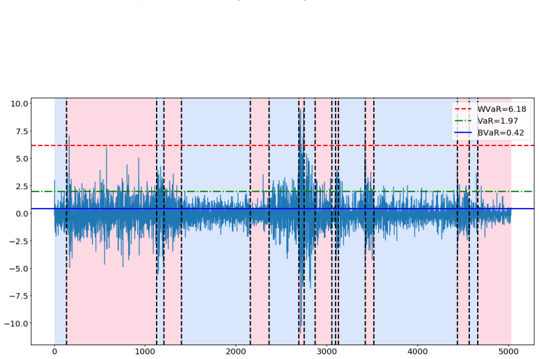
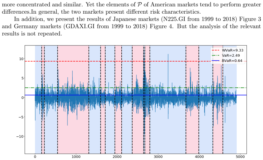
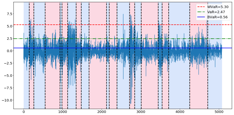
The central claim is that WVaR under model uncertainty can be computed empirically from Eq. 18: after segmenting the return series and fitting a two-layer Gaussian mixture whose per-segment weights $\beta_j^{(t)}$ vary but whose first-layer components $p_j(r|\theta_j)$ are shared across segments, the uncertainty set is $\mathcal{P}=\{p_j: j=1,\dots,K_2\}$ and the worst-case VaR is $WVaR_\alpha(X)=-\inf\{x: \max_j P_{p_j}[X\le x]>\alpha\}$, the largest VaR among the estimated market factors. The paper further argues that a one-layer Gaussian mixture with the same total number of components would overestimate this worst-case value, because the maximum over individual normal components can exceed the maximum over the grouped market-factor distributions; the two-layer structure is therefore not a cosmetic choice but a substantive constraint on which distributions count as possible models. The paper applies the construction to four markets, reporting WVaR, VaR, and BVaR figures for each.

Load-bearing premise

The whole calculation rests on the assumption that the true set of possible models is exactly the finite set of estimated first-layer market-factor distributions and that those factors stay fixed across time, so if those factors drift or the set should contain other distributions, the computed worst-case VaR is not the true worst case.

Editorial extensions

If this is right

For the Chinese and US indices reported in detail, ignoring model uncertainty understates tail risk: WVaR is roughly twice the ordinary VaR (5.89% vs 2.59% and 6.18% vs 1.97%).
The US market has a higher worst-case VaR than the Chinese market even though its ordinary VaR is lower, which the paper reads as evidence that the US factor distributions are more spread out and that the i.i.d. assumption is unsuitable for tail measurement.
The worst scenario is a single market-factor distribution, not a mixture, so the computed WVaR comes with a concrete interpretation of which factor drives the extreme loss.
A one-layer Gaussian mixture with more components would overstate the worst-case VaR, so the two-layer structure is the recommended choice for empirical worst-case bounds.

Reading between the lines

Editorial extensions of the paper, not claims the author makes directly.

The same finite-uncertainty-set construction would apply to expected shortfall or any law-invariant risk measure, not just VaR; the paper only computes quantile-based bounds.
The stability of the first-layer factors is testable: refitting the model on rolling windows and comparing the estimated component parameters would reveal whether the fixed set $\mathcal{P}$ is credible or whether WVaR should be calculated over a larger family.
Treating the first-layer weights themselves as uncertain would enlarge the uncertainty set and push WVaR upward, so the reported numbers should be read as the minimal worst case under the paper's assumptions, not a universal upper bound.
The predicted one-layer overestimation could be checked directly by fitting both models to the same data and comparing WVaR values; a large gap would indicate that the grouping into market factors is doing real work.

Share X Bluesky LinkedIn Reddit HN

Signed reviews

No signed human review yet.

Editorial analysis

A structured set of objections, weighed in public.

Desk editor's note, referee report, and a circularity audit.

Desk Editor's Note

read the letter

Quick take. The paper has a real modeling idea—market factors as mixture components whose weights are uncertain—and the empirical application is a useful illustration. But the EM M-step in Eq. 69 breaks the model's own normalization constraint, so the reported WVaR numbers are not supported by the derivation. The reader's conditional verdict is in the right neighborhood, but the normalization issue is a hard flaw, not a validation gap.

What's new and worth credit: the two-layer Gaussian mixture with change-point segmentation is a genuine twist on the standard GMM/VaR approach. The first layer carries financial meaning (market factors), the second layer is numerical scaffolding. The paper is honest about the difficulty of estimating model uncertainty, and the four-market comparison gives a concrete sense of how WVaR can exceed VaR. The EM and change-point machinery are standard and mostly assembled correctly.

The soft spots are serious. Eq. 69 gives the M-step for α_{j,i} as (K2/\bar N) Σ_t \bar n^t_{j,i}, which enforces only the global sum over all j,i, not the per-component constraint Σ_i α_{j,i}=1 required for p_j to be a density. With K2=5, the within-j sums will generally drift from 1, so the CDFs entering the WVaR definition (Eq. 18) are not well-defined. The correct update is A_{j,i}/Σ_i A_{j,i}. Unless the implementation silently renormalizes, the headline numbers 5.89% and 6.18% don't follow from the model as written. The parameter choices (K1=3, K2=5, β=2.5) are ad hoc, with no sensitivity analysis or out-of-sample validation. The argument that the two-layer model avoids overestimation relative to a one-layer GMM is informal. Also, the paper claims no prior empirical WVaR results, but cites Peng et al. [45], which appears to do exactly that.

None of this kills the underlying recipe; the normalization error is fixable, and the sensitivity concerns can be addressed with a modest additional study. But in its current form the paper is not a reliable source for the numerical worst-case figures.

I would send it to peer review, expecting major revision. The referee should check the EM derivation first, then ask for sensitivity analysis and an out-of-sample exercise. For a reading group, it's a maybe—good for practicing derivation-checking, not as a reference. I wouldn't cite it yet.

Referee Report

5 major / 5 minor

Summary. The paper proposes a two-layer Gaussian mixture model for financial returns in which the first-layer components represent market factors and are themselves Gaussian mixtures, while the segment-level mixing weights are allowed to vary across change-point segments. The model uncertainty set P is effectively taken to be the estimated first-layer component distributions. Returns are segmented with a kernel-based change-point detector, parameters are estimated by EM, and worst-case and best-case Value-at-Risk are computed as the maximum and minimum VaR over the estimated component distributions. Empirical values are reported for Chinese, US, Japanese, and German index return series.

Significance. If correct, the paper would be one of the few empirical implementations of worst-case VaR under model uncertainty, and the two-layer construction gives a practical way to build a finite candidate set from data. The use of change-point segmentation with mixture components shared across segments is a sensible way to capture nonstationarity while keeping an interpretable set of market factors. The paper is honest about the limited scope of its uncertainty set and provides a concrete computational recipe. However, the paper provides no code, no convergence diagnostics, and no out-of-sample validation; and, as detailed below, a key M-step equation is not the correct maximizer under the model's normalization constraints. The claimed numerical WVaR values are therefore not supported by the derivation as written.

major comments (5)

[Section 5, Eq. (69)] The update for the shared mixture weights α_{j,i} is not the maximizer of Q under the constraints Σ_i α_{j,i}=1 for each j. From Eq. (65), the α-dependent part of Q is Σ_{j,i} A_{j,i} log α_{j,i} with A_{j,i}=Σ_t \bar n^t_{j,i}; the correct M-step is \hat α_{j,i}=A_{j,i}/Σ_i A_{j,i}. Eq. (69) instead enforces only the global sum Σ_{j,i} α_{j,i}=K2, so the fitted p_j(r|θ_j) need not integrate to one. Consequently the CDFs entering the WVaR definition in Eq. (18) are undefined, and the reported WVaR_SH=5.89% and WVaR_SP=6.18% are unsupported unless the implementation silently renormalizes. Please correct the formula and rerun, or report the normalization actually used.
[Section 6, hyperparameter choices] The number of second-layer components K2=5, the number of first-layer components K1=3, the change-point penalty β=2.5, and the Gaussian-kernel bandwidth γ are introduced without justification or sensitivity analysis. Because WVaR in Eq. (18) is a maximum over the K2 estimated component distributions, the reported WVaR values depend directly on the arbitrary choice K2=5; a different choice can change the maximum. Please provide model selection, a sensitivity study, or at least a discussion of how the results vary with these parameters.
[Section 3, Eq. (18)] The uncertainty set P is never defined precisely. If P is the set of all mixtures of the estimated component distributions with unknown first-layer weights, Eq. (18) follows because max over the simplex of Σ_j β_j F_j(x) is max_j F_j(x); if P is only the finite set of the K2 estimated component distributions, the claimed representation of model uncertainty is not the one described in Section 3. This ambiguity affects the interpretation of the WVaR numbers and should be resolved explicitly.
[Section 6, validation] The title and abstract describe a prediction procedure, but Section 6 only reports in-sample statistics on the full 1999-2018 sample. There is no backtest, holdout period, or comparison with a benchmark prediction method, so the empirical claims (e.g., that American markets have a more severe worst-case than the Chinese market) are not validated. Please add an out-of-sample exercise or change the language from 'prediction' to 'estimation'.
[Section 3, Eqs. (32)-(38)] The argument that the two-layer model avoids overestimation relative to a one-layer Gaussian mixture model is informal. The sketch considers a single component of the worst first-layer distribution as the one-layer 'worst' distribution, but the one-layer model's uncertainty set is not defined, and inequality (37) alone does not show that the one-layer WVaR is always at least as large. Please give a precise statement with the candidate sets for both models, or weaken the claim.

minor comments (5)

[Section 3, Eq. (10) and Section 5, Eq. (56)] The symbol N is used both for the number of segments and for the total sample size, which is confusing; please use distinct notation, e.g., m for the number of segments and n for the total number of observations.
[Section 3, Eq. (18)] The expression 'maxPpj[X≤x]' is malformed; write max_{j=1,...,K2} P_{p_j}[X≤x] and define the set over which the maximum is taken.
[Abstract and Introduction] The manuscript contains numerous typos and grammatical errors (e.g., 'the the family of models', 'simply the P to a set'), and the English needs careful editing throughout.
[Section 6, empirical results] Only point estimates of WVaR, VaR, and BVaR are reported; please include the number of segments, the estimated component parameters, and some measure of estimation uncertainty (e.g., standard errors or bootstrap intervals) for reproducibility.
[References] Some references are incomplete or inconsistent (e.g., page ranges, journal names), and the list should be checked against the journal's style.

Circularity Check

0 steps flagged · score 0.0 of 10

No significant circularity: the WVaR values are direct applications of Definition 2.2 to likelihood-fitted component distributions, not fitted-to-target predictions.

full rationale

The paper's chain is: assume a two-layer Gaussian mixture per segment (Eqs. 11-28); define the uncertainty set as the first-layer components p_j(r|theta_j) (Eq. 18); estimate the component parameters by EM maximizing the observed-data likelihood (Eqs. 60-69); then compute WVaR as the maximum VaR over the estimated p_j. The WVaR is therefore a deterministic functional of the fitted model, but it is not a fitted parameter renamed as a prediction: the EM objective (Eq. 65) is the log-likelihood, not the WVaR, so the reported values 5.89% and 6.18% are not optimized to match any outcome. The set P in Eq. 18 is a modeling assumption (the market-factor components are assumed constant with only segment weights varying), not a result derived from the data; this weakens the external validity of the 'worst-case' label, but a modeling assumption is not circularity. The comparison in Eqs. 32-38 showing that a one-layer mixture overestimates WVaR is a mathematical inequality about quantiles of mixtures, not a step that imports the conclusion. No uniqueness theorem or load-bearing self-citation is used; the citation to Peng[45] is contextual and does not justify the model choice. One substantive mathematical flaw exists in Eq. 69: the M-step update for alpha_{j,i} does not enforce the per-component normalization sum_i alpha_{j,i}=1, so the estimated p_j may not be densities and the numerical WVaR values are unsupported. This is an internal-consistency and correctness problem, not a circularity, because the flaw does not make the output equivalent to an input; it makes the computation invalid under the model's own constraints.

Assumptions & free parameters 5 free parameters · 4 assumptions · 0 invented entities

The central WVaR calculation rests on several free parameters (K1, K2, β, γ, EM initialization) and on the domain assumptions that market factors are time-invariant and that the uncertainty set comprises the estimated components. None of these are validated by model selection, sensitivity analysis, or external data.

free parameters (5)

K1 = 3
Number of second-layer Gaussian components, chosen by hand without model selection or sensitivity analysis.
K2 = 5
Number of first-layer market factors, chosen by hand without model selection or sensitivity analysis.
Beta (change point penalty) = 2.5
Smoothing parameter in the linear penalty for change point detection, set to 2.5 with no justification or sensitivity analysis.
Gamma (kernel bandwidth) = Not stated
Bandwidth of the Gaussian kernel in change point detection, mentioned in Eq. (43) but its value is not reported.
EM initialization = Not stated
Initial values for means, variances, and weights in the EM algorithm are not specified, which can affect the fitted components and hence WVaR.

assumptions (4)

domain assumption Within each segment Rt, the returns are independent and identically distributed.
Stated in Section 3 and used to justify fitting a single mixture distribution per segment.
domain assumption The first-layer component distributions p_j(r|θ_j) (market factors) are time-invariant; only the weights β_t_j change across segments.
Assumed in Section 3 after Eq. (17) so that a single set of component parameters can be estimated from all segments.
ad hoc to paper The model uncertainty set P is exactly the set of the K2 estimated market-factor distributions, not all mixtures of them.
Eq. (18) defines WVaR as the maximum over the component distributions p_j, which presumes the market factors themselves are the possible models, a strong modeling choice.
domain assumption The change point detection method with a linear penalty correctly identifies the segments where the i.i.d. assumption holds.
Section 4 relies on the ruptures implementation and the chosen penalty without testing the segmentation quality.

how reviews work

0 comments

Cite this review

Pith. "Pith review of calculation worst-case Value-at-Risk prediction using empirical data under model uncertainty." pith.science (2026). https://pith.science/paper/HDZ2LFNG

@misc{pith2026190800982,
  author       = {Pith},
  title        = {Pith review of: calculation worst-case Value-at-Risk prediction using empirical data under model uncertainty},
  year         = {2026},
  howpublished = {\url{https://pith.science/paper/HDZ2LFNG}},
  note         = {Machine review of arXiv:1908.00982}
}

abstract

Quantification of risk positions under model uncertainty is of crucial importance from both viewpoints of external regulation and internal management. The concept of model uncertainty, sometimes also referred to as model ambiguity. Although we know the family of models, we cannot precisely decide which one to use. Given the set $\mathcal{P}$, the value of the risk measure $\rho$ varies in a range over the set of all possible models. The largest value in such a range is referred to as a worst-case value, and the corresponding model is called a worst scenario. Value-at-Risk(VaR) has become a very popular risk-measurement tool since it was first proposed. Naturally, WVaR(worst-case Value-at-Risk) attracts the attention of many researchers. Although many literatures investigated WVaR, the implications for empirical data analysis remain rare. In this paper, we proposed a special model uncertainty market model to simply the $\mathcal{P}$ to a set contain finite number of probability distributions. The model has the structure of the two-layer mixed distribution model. We used change point detection method to divide the returns series and then used EM algorithm to estimate the parameters. Finally, we calculated VaR, WVaR(worst-case Value-at-Risk) and BVaR(best-case Value-at-Risk) for four financial markets and then analyzed their different performance.

Figures

Figures reproduced from arXiv: 1908.00982 by the authors.

**Figure 2.** American(SPX.GI) financial market 12 [PITH_FULL_IMAGE:figures/full_fig_p012_2.png] view at source ↗

**Figure 3.** Japanese(N225.GI) financial market 7 Conclusion With the rapid development of the financial industry and the frequent emergence of financial crisis, risk management has become an important issue faced by company managers and government regulators. Nowadays, quantification of risky positions held by a financial institution under model uncertainty is of crucial importance from both viewpoints of external regulation a… view at source ↗

Figures from the paper (1 more)

**Figure 4.** Figure 4: Germany(GDAXI.GI) financial market component distributions correspond to different market factors. The weights of components represent the probability of the occurrence of market factors. We don’t care about and unable to model the probability of the occurrence of com…

Discussion (0). Continue with ORCID to comment.

Reference graph

Works this paper leans on

48 extracted references · 41 canonical work pages

[45]

Improving Value-at-Risk prediction under model uncertainty

Peng S, Yang S Z, and Yao J F. Improving value-at-risk prediction under model uncertainty. Working paper, Shandong University, arXiv:1805.03890 , 2018

work page Pith review arXiv 2018
[1]

An overview of value at risk

Duﬃe D and Pan J. An overview of value at risk. Journal of Derivatives , 4(3):7–49, 1997

1997
[2]

Techniques for verifying the accuracy of risk measurement models

Kupiec P. Techniques for verifying the accuracy of risk measurement models. Journal of Derivatives, 2(2):73–84, 1995

1995
[3]

Evaluating interval forecasts

Christoﬀersen P-F. Evaluating interval forecasts. International Economic Review, 39(4):841– 862, 1998

1998
[4]

Risk Management and Financial Institutions (3rd Edition)

Hull J. Risk Management and Financial Institutions (3rd Edition) . John Wiley & Sons,, 2012

2012
[5]

Craig Mackinlay

Andrew W Lo and A. Craig Mackinlay. Stock market prices do not follow random walks: Evidence from a simple speciﬁcation test. Review of Financial Studies , 1(1):41–66, 1988

work page 1988
[6]

The impact of stationarity assessment on studies of volatility and value-at-risk

Leskow J. The impact of stationarity assessment on studies of volatility and value-at-risk. Mathematical & Computer Modelling , 34(9):1213–1222, 2001

work page 2001
[7]

An improved methodology for measuring var

Zangari P. An improved methodology for measuring var. Riskmetrics Monitor, 1996

work page 1996

Show all 48 references

[8]

Value at risk for a mixture of normal distributions: the use of quasi-bayesian estimation techniques

Venkataraman S. Value at risk for a mixture of normal distributions: the use of quasi-bayesian estimation techniques. Economic Perspectives, 21(2):2–13, 1997

1997
[9]

Measuring risk in value-at-risk based on students t-distribution

Huschens S and Kim J R. Measuring risk in value-at-risk based on students t-distribution. 1999

1999
[10]

Portfolio valueatrisk with heavytailed risk factors

Glasserman P, Heidelberger P, and Shahabuddin P. Portfolio valueatrisk with heavytailed risk factors. Mathematical Finance, 12(3):239–269, 2002

2002
[11]

Can the student-t distribution provide accurate value at risk? Journal of Risk Finance, 7(3):292–300, 2006

Lin C H and Shen S S. Can the student-t distribution provide accurate value at risk? Journal of Risk Finance, 7(3):292–300, 2006

2006
[12]

Value at risk based on the volatility, skewness and kurtosis

Li D X. Value at risk based on the volatility, skewness and kurtosis. Riskmetrics Group, 1999

1999
[13]

Value at risk with time varying variance, skewness and kurtosis-the nig-acd model

Wilhelmsson A. Value at risk with time varying variance, skewness and kurtosis-the nig-acd model. Econometrics Journal, 12(1):82–104, 2010

2010
[14]

Empirical analysis of jump dynamics, heavy-tails and skewness on value-at-risk estimation

Su J B and Hung J C. Empirical analysis of jump dynamics, heavy-tails and skewness on value-at-risk estimation. Economic Modelling, 28(3):1117–1130, 2011

2011
[15]

Forecasting value-at-risk with time-varying variance, skewness and kurtosis in an exponential weighted moving average framework

Gabrielsen A, Kirchner A, Liu Z S, and Zagaglia P. Forecasting value-at-risk with time-varying variance, skewness and kurtosis in an exponential weighted moving average framework. Mpra Paper, 10(1), 2012

2012
[16]

Improved duration-based backtesting of value-at-risk

H Markus. Improved duration-based backtesting of value-at-risk. Social Science Electronic Publishing, 8(2), 2006

2006
[17]

Comparison of certain value-at-risk estimation methods for the two-parameter weibull loss distribution

Gebizlioglu O L, Senoglu B, and Kantar Y M. Comparison of certain value-at-risk estimation methods for the two-parameter weibull loss distribution. Journal of Computational & Applied Mathematics, 235(11):3304–3314, 2011

2011
[18]

Value at risk when daily changes in market variables are not normally distributed

Hull J C and White A D. Value at risk when daily changes in market variables are not normally distributed. Journal of Derivatives , 5(3):9–9, 1998. 15

1998
[19]

An approach to var for capital markets with gaussian mixture

Zhang M H and Cheng Q S. An approach to var for capital markets with gaussian mixture. Applied Mathematics & Computation , 168(2):1079–1085, 2005

2005
[20]

Value-at-risk: a multivariate switching regime approach

Billio M and Pelizzon L. Value-at-risk: a multivariate switching regime approach. Journal of Empirical Finance, 7(5):531–554, 2000

2000
[21]

Value-at-risk in a market subject to regime switching

Kawata R and Kijima M. Value-at-risk in a market subject to regime switching. Quantitative Finance, 7(6):609–619, 2007

2007
[22]

Value-at-risk prediction: A comparison of alternative strategies

Kuester K, Mittnik S, and Paolella M S. Value-at-risk prediction: A comparison of alternative strategies. Journal of Financial Econometrics , 4(1):53–89, 2006

2006
[23]

Risk management

Jorion P. Risk management. Annual Review of Financial Economics , 2(1):347–365, 2010

2010
[24]

A comprehensive review of value at risk methodologies

Abad P, Benito S, and Lopez C. A comprehensive review of value at risk methodologies. Spanish Review of Financial Economics , 12(1):15–32, 2014

2014
[25]

A review of backtesting for value at risk

Zhang Y and Nadarajah S. A review of backtesting for value at risk. Communication in Statistics-Theory and Methods, 47(15), 2017

2017
[26]

Bayesian Inference: Kendall’s Advanced Theory of Statistics

O’Hagan A. Bayesian Inference: Kendall’s Advanced Theory of Statistics . London: Edward Arnold, 1994

1994
[27]

BayesianTheory

Bernardo J M and Smith A F M. BayesianTheory. Chichester, UK: Wiley, 1994

1994
[28]

Quantile uncertainty and value-at-risk model risk.Risk Analysis, 32(8):1293–1308, 2012

Alexander C and Sarabia J M. Quantile uncertainty and value-at-risk model risk.Risk Analysis, 32(8):1293–1308, 2012

2012
[29]

Estimation of upper quantiles under model and parameter uncertainty

Modarres R, Nayak T K, Gastwirth J L, and Azen S P. Estimation of upper quantiles under model and parameter uncertainty. Computational Statistics & Data Analysis , 39(4):529–554, 2007

2007
[30]

Uncertainty of quantile estimates in the measurement of self-similar processes

Giorgi G and Narduzzi C. Uncertainty of quantile estimates in the measurement of self-similar processes. In IEEE International Workshop on Advanced Methods for Uncertainty Estimation in Measurement, 2008

2008
[31]

Estimation error in the assessment of ﬁnancial risk exposure

Figlewski S. Estimation error in the assessment of ﬁnancial risk exposure. Social Science Electronic Publishing, 112(D1):107–119, 2003

2003
[32]

Measuring the risk in value at risk

Jorion P. Measuring the risk in value at risk. Financial Analysts Journal , (52):47–56, 1996

1996
[33]

Worst case model risk management

Talay D and Zheng Z Y. Worst case model risk management. Finance & Stochastics, 6(4):517– 537, 2002

2002
[34]

Model uncertainty and its impact on the pricing of derivative instruments

Cont R. Model uncertainty and its impact on the pricing of derivative instruments. Mathe- matical Finance, 16(3):519547, 2006

2006
[35]

Bounds on a distribution function when its ﬁrst n moments are given

Royden H L. Bounds on a distribution function when its ﬁrst n moments are given. Annals of Mathematical Statistics, 24(3):361–376, 1953

1953
[36]

Best bounds for positive distribution with ﬁxed moments

Kaas R and Goovaerts M. Best bounds for positive distribution with ﬁxed moments. Insurance: Mathematics & Economics , (5):87–92, 1984. 16

1984
[37]

How to estimate the value at risk under incomplete information

De Schepper A and Heijnen B. How to estimate the value at risk under incomplete information. Journal of Computational & Applied Mathematics , 233(9):2213–2226, 2010

2010
[38]

A semideﬁnite programming approach to optimal-moment bounds for convex classes of distributions

Popescu I. A semideﬁnite programming approach to optimal-moment bounds for convex classes of distributions. Mathematics of Operations Research, (30):623–657, 2005

2005
[39]

Bounding probability of small deviation: A fourth moment approach

He S, Zhang J, and Zhang S. Bounding probability of small deviation: A fourth moment approach. Mathematics of Operations Research, (35):208–232, 2010

2010
[40]

Filtration consistent nonlinear expectations and evaluations of contingent claims

Peng S. Filtration consistent nonlinear expectations and evaluations of contingent claims. Acta Mathematicae Applicatae Sinica, (20):1–24, 2004

2004
[41]

g- expectation, g-brownian motion and related stochastic calculus of ito type

Peng S. Stochastic analysis and applications: The abel symposium 2005, chapter “g- expectation, g-brownian motion and related stochastic calculus of ito type”. Springer, Berlin Heidelberg, 2006

2005
[42]

Multi-dimensional g-brownian motion and related stochastic calculus under g- expectation

Peng S. Multi-dimensional g-brownian motion and related stochastic calculus under g- expectation. Stochastic Processes and Their Applications , (118):2223–2253, 2008

2008
[43]

Nonlinear expectations and stochastic calculus under uncertainty

Peng S. Nonlinear expectations and stochastic calculus under uncertainty. Technical report, Shandong University, arXiv:1002.4546v1 , 2010

2010 arXiv
[44]

Coherent measures of risk

Artzner P, Delbaen F, Eber J-M, and Heath D. Coherent measures of risk. Mathematical Finance, 9(3):203–228, 1999

1999
[46]

Retrospective mutiple change point estimation with kernels

Harchaoui Z and Cappe O. Retrospective mutiple change point estimation with kernels. In IEEE/SP Workshop on Statistical Signal Processing , 2007

2007
[47]

Selective review of oﬄine change point detection methods

Charles T, Laurent O, and Nicolas V. Selective review of oﬄine change point detection methods. arXiv:1801.00718v2, 2018

2018 arXiv
[48]

ruptures: change point detection in python

Charles T. ruptures: change point detection in python. In URL http:// ctruong.perso.math.cnrs.fr/ruptures. [Online]., 2018. 17

2018

Pith tools

Reviewed August 14, 2026 · model on record in the stance chip above.

[1] [45]

Improving Value-at-Risk prediction under model uncertainty

Peng S, Yang S Z, and Yao J F. Improving value-at-risk prediction under model uncertainty. Working paper, Shandong University, arXiv:1805.03890 , 2018

work page Pith review arXiv 2018

[2] [1]

An overview of value at risk

Duﬃe D and Pan J. An overview of value at risk. Journal of Derivatives , 4(3):7–49, 1997

1997

[3] [2]

Techniques for verifying the accuracy of risk measurement models

Kupiec P. Techniques for verifying the accuracy of risk measurement models. Journal of Derivatives, 2(2):73–84, 1995

1995

[4] [3]

Evaluating interval forecasts

Christoﬀersen P-F. Evaluating interval forecasts. International Economic Review, 39(4):841– 862, 1998

1998

[5] [4]

Risk Management and Financial Institutions (3rd Edition)

Hull J. Risk Management and Financial Institutions (3rd Edition) . John Wiley & Sons,, 2012

2012

[6] [5]

Craig Mackinlay

Andrew W Lo and A. Craig Mackinlay. Stock market prices do not follow random walks: Evidence from a simple speciﬁcation test. Review of Financial Studies , 1(1):41–66, 1988

work page 1988

[7] [6]

The impact of stationarity assessment on studies of volatility and value-at-risk

Leskow J. The impact of stationarity assessment on studies of volatility and value-at-risk. Mathematical & Computer Modelling , 34(9):1213–1222, 2001

work page 2001

[8] [7]

An improved methodology for measuring var

Zangari P. An improved methodology for measuring var. Riskmetrics Monitor, 1996

work page 1996