REVIEW 2 major objections 4 minor 40 references
Introduction to nonlinear discrete systems: Theory and modeling
T0 review · 2 major / 4 minor · reviewed 2026-08-14 · deepseek-v4-flash
Pith's one-line read This paper proposes a self-contained, code-backed introduction to nonlinear discrete systems built on the DNLS equation, and argues that the same analytical and numerical sequence transfers to other lattice models.
desk verdict A useful teaching tutorial on the DNLS equation, but Eq. (2) contains a real sign error that makes Problem 3 ask students to prove a false invariant. read the letter →
The pith
A machine-rendered reading of the paper's core claim, the machinery that carries it, and where it could break.
The reading
What carries the argument
The load-bearing object is the discrete nonlinear Schrödinger (DNLS) equation, a nearest-neighbor lattice model with cubic onsite nonlinearity. The argument is carried by a small set of ansätze: the plane wave $u_k=a\,e^{i(qk-\omega t)}$ for dispersion, the modulated plane wave $u_k=(a+b_k(t))e^{i(qk-\omega t)}$ for modulational instability, the stationary mode $u_k=U_k e^{-i\eta t}$ for solitons, and the perturbed stationary mode $u_k=(U_k+w_k(t))e^{-i\eta t}$ for stability. Substituting each ansatz and linearizing in the small quantities reduces the problem to algebraic or eigenvalue equations, and the anti-continuum limit provides the localized seed that the Newton-Raphson solver (Mathematica's FindRoot) needs. The stability verdict is read from the complex frequencies of the final eigenvalue problem: any nonzero imaginary part means instability.
What would settle it
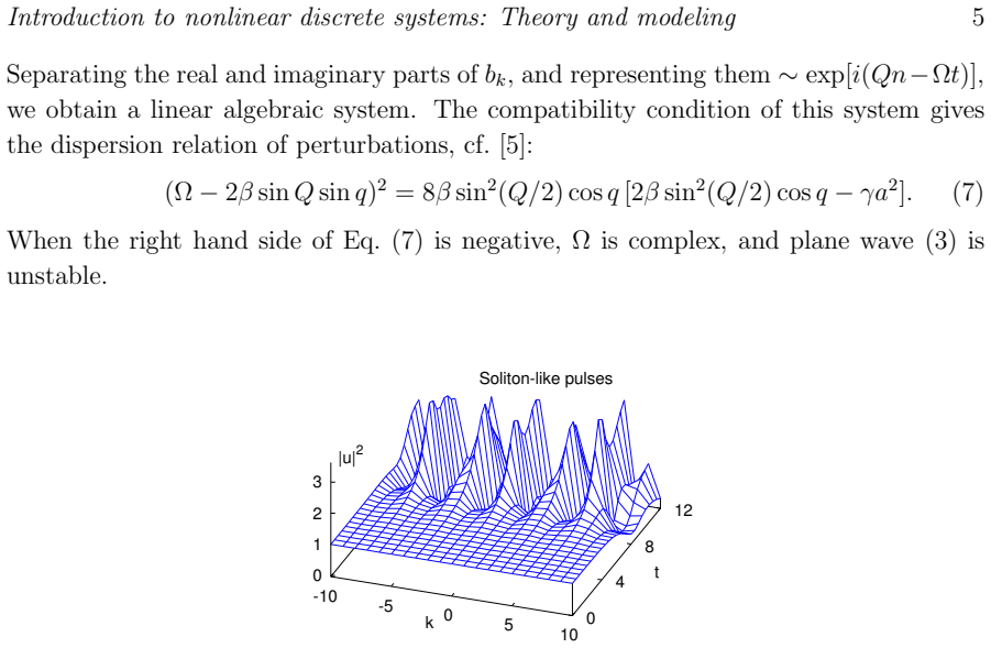
Run the supplied Mathematica code with $\beta=0.5$, $\gamma=1$, and $\eta=-2$: the on-site soliton should stay stationary with maximum imaginary part of the modulation eigenvalues around $10^{-7}$, the inter-site soliton should be unstable, and a noise-modulated plane wave with $\epsilon=10^{-3}$ should break into soliton-like pulses; failure of any of these outputs would show the tutorial does not deliver its central claim.
Extended reading notes
Core claim
The authors claim that the main ideas and methods of nonlinear discrete-system theory can be presented through the DNLS equation $i\,du_k/dt + \beta(u_{k+1}+u_{k-1}) + \gamma|u_k|^2u_k=0$, and that the analysis sequence is generic. They derive the plane-wave dispersion relation $\omega = -(2\beta\cos q + \gamma a^2)$, the modulational-instability condition $(\Omega - 2\beta\sin Q\sin q)^2 = 8\beta\sin^2(Q/2)\cos q\,[2\beta\sin^2(Q/2)\cos q - \gamma a^2]$, the stationary soliton equation $-\beta(U_{k+1}+U_{k-1}) - \gamma|U_k|^2U_k = \eta U_k$, and a linear-stability eigenvalue problem for small perturbations. The paper also uses the continuous limit and the anti-continuum limit $\beta=0$ to construct soliton approximations, and supplies Mathematica code covering every one of these steps.
Load-bearing premise
The load-bearing premise is that the toolkit demonstrated on the DNLS equation is generic enough to transfer to other discrete systems, which the paper asserts in Section 4 but does not demonstrate in detail.
Editorial extensions
If this is right
- A student who follows the paper and runs the Mathematica code can reproduce the dispersion relation, the modulational-instability growth, and the soliton stability spectra for the stated parameters.
- The same five-step sequence (plane wave, dispersion, modulational instability, stationary soliton, linear stability) can be applied to other discrete systems, as the paper claims in Section 4 and demonstrates via the suggested problems.
- The code is written for nearest-neighbor equations and can be extended to more general couplings, different nonlinearities, and higher-dimensional arrays.
- Modulational instability of a nonlinear plane wave leads to break-up into soliton-like pulses, which is how the paper motivates the relevance of discrete solitons.
Reading between the lines
- The Mathematica code could be refactored into a reusable template: changing the coupling term and nonlinearity in MC.1 and re-running MC.2–MC.10 would give a working stability analysis for other lattice models without re-deriving the linear algebra.
- The eigenvalue formulation suggests a natural extension to two- and three-dimensional arrays by altering the neighbor indexing in the code, a step the paper mentions but does not carry out.
- The paper's implicit pedagogical claim is testable: comparing students who work through this DNLS pipeline against students who only see linear lattice theory would show whether the nonlinear toolkit transfers as claimed.
- Because the anti-continuum limit provides the numerical seed, the method is especially well suited to strongly localized modes, which is where discrete effects differ most from continuum solitons.
Signed reviews
Editorial analysis
A structured set of objections, weighed in public.
Referee Report
Summary. The manuscript proposes a pedagogical introduction to nonlinear discrete systems, using the discrete nonlinear Schrödinger (DNLS) equation as a universal model. It covers plane-wave dispersion, modulational instability, discrete bright solitons, the anti-continuum limit, numerical construction of stationary solitons, and linear stability analysis, and it supplies a Mathematica script together with twelve problems. The paper is aimed at university courses and claims to provide a self-contained analytical and numerical toolkit that can be extended to other discrete systems.
Significance. If corrected, this would be a useful teaching resource for Eur. J. Phys.: the analytical derivations are standard, the Mathematica code is provided as a working supplement, and the problems extend the methods to impurity modes, surface modes, cubic-quintic, and Ablowitz-Ladik/Salerno models. The modulational-instability condition and the linear stability equations are consistent with the literature, and the code appears to reproduce known results. The paper does not claim new research results; its value lies in accessibility and reproducibility, which are genuine strengths.
major comments (2)
- [Eq. (2), §3 Problem 3] The Hamiltonian H in Eq. (2) is not an invariant of Eq. (1). With β0=0, differentiating H = Σ[β|u_k-u_{k-1}|² + (γ/2)|u_k|⁴] along the flow gives a generally nonzero result. For a periodic N=4 chain with β=γ=1 and initial condition (1,2i,0,0), direct differentiation using Eq. (1) gives dH/dt=24. The correct conserved quantity is H' = Σ[β0|u_k|² + β|u_k-u_{k-1}|² - (γ/2)|u_k|⁴]. Because Problem 3 explicitly asks students to prove that P and H in Eq. (2) are invariants, this is a load-bearing error that must be corrected.
- [Sec. 2.2, Eq. (8)] The continuum limit is misstated by a factor of two. Using the intended phase transformation u_k = w(x_k,t) e^{2iβt} and expanding u_{k+1}+u_{k-1} ≈ 2u_k + h²∂²u/∂x² in Eq. (1) gives i w_t + βh² w_xx + γ|w|²w = 0, not 2βh². Equation (9) is consistent with the coefficient β (for h=1), so Eq. (8) should be corrected, and the missing imaginary unit in the transformation w ≈ u_k exp(−2βt) should also be fixed.
minor comments (4)
- [Abstract and §1] The phrase 'nonlinear distributed systems' should read 'nonlinear discrete systems'; the paper treats discrete lattices, not distributed (continuum) systems.
- [Sec. 2.2, first sentence] The statement 'There is no exact DS solutions of the DNLS equation' is too absolute and should be qualified, for example as 'no exact closed-form bright-soliton solutions in the general nonintegrable case', since integrable variants such as the Ablowitz-Ladik equation in Problem 11 do possess exact soliton solutions.
- [Problem 5, §3] Typographical error: 'staggered solions' should be 'staggered solitons'.
- [Eq. (9), Sec. 2.2] The soliton width in Eq. (9) is written without the lattice spacing h; if h is retained, the width should be ν = h√(2β)/(A√γ).
Circularity Check
No significant circularity: all derivations are self-contained and no prediction reduces to a fitted input.
full rationale
The paper's analytical chain is carried out explicitly inside the manuscript: the dispersion relation (4) follows from substituting the plane-wave ansatz (3) into Eq. (1); the modulational-instability condition (7) follows from linearizing the perturbed solution (5); the stationary soliton equation (11) follows from the substitution uk(t)=Uk exp(-i eta t); and the stability analysis follows from linearizing around the numerically found soliton profile. No parameter is fitted to a subset of data and then used to predict a closely related quantity, and no 'prediction' is defined in terms of the model input. Citations to the DNLS literature are contextual or problem-suggesting rather than load-bearing derivations. The only self-citation by an author of this paper is reference [23] in Problem 10, and it is used only as a pointer for study, not as a justification of the paper's central claim. The suspected sign error in the Hamiltonian H in Eq. (2) is a correctness concern, not a circularity concern: Problem 3 asks students to verify the invariant, so the invariant is not being used as an input to derive the result. Because the derivations are self-contained, code-reproducible, and compared against known textbook results, no circular step is present.
Assumptions & free parameters
assumptions (3)
- domain assumption The DNLS equation (1) is a valid model for the physical systems listed: waveguide arrays, BEC in optical lattices, Josephson junction arrays, and others.
- domain assumption Any initial field distribution with finite power P eventually splits into spreading waves and discrete solitons, justifying the focus on these modes.
- standard math Newton-Raphson iteration converges to a physical soliton profile for the chosen initial conditions.
Cite this review
Pith. "Pith review of Introduction to nonlinear discrete systems: Theory and modeling." pith.science (2026). https://pith.science/paper/MHIWZMJJ
@misc{pith2026190801497,
  author       = {Pith},
  title        = {Pith review of: Introduction to nonlinear discrete systems: Theory and modeling},
  year         = {2026},
  howpublished = {\url{https://pith.science/paper/MHIWZMJJ}},
  note         = {Machine review of arXiv:1908.01497}
}
read the original abstract
An analysis of discrete systems is important for understanding of various physical processes, such as excitations in crystal lattices and molecular chains, the light propagation in waveguide arrays, and the dynamics of Bose-condensate droplets. In basic physical courses, usually linear properties of discrete systems are studied. In this paper we propose a pedagogical introduction to the theory of nonlinear distributed systems. The main ideas and methods are illustrated using a universal model for different physical applications, the discrete nonlinear Schr\"{o}dinger (DNLS) equation. We consider solutions of the DNLS equation and analyze their linear stability. The notions of nonlinear plane waves, modulational instability, discrete solitons and the anti-continuum limit are introduced and thoroughly discussed. A Mathematica program is provided for better comprehension of results and further exploration. Also, few problems, extending the topic of the paper, for independent solution are given.
Figures


Figures from the paper (1 more)

Reference graph
Works this paper leans on
-
[1]
Introduction A discrete system is a system that consists of several (or an infinit e number of) well- separated points (sites). Each site is characterized by some varia bles, so that at a given time these variables specify a state of the system. A change of var iables on each site may depend on values on other sites. Many important physical systems, such a...
-
[2]
Analysis of waves in discrete systems 2.1. Plane waves For discrete systems, it is instructive to start the analysis from a p lane wave solution. We look for a solution in the following form: uk(t) = a exp[i(qk − ωt)], (3) where a, q, and ω are the amplitude, the wave number and the frequency of the plane wave. A substitution of Eq. (3) into Eq. (1) resul...
-
[3]
Questions and Problems In this Section, we suggest few problems. The aim of the problems is t o help a deeper understanding of the methods reviewed in this paper, and a lso to develop skills in working with Mathematica program in Appendix A. Problems 1-7 c onsider the fundamental properties of plane waves and solitons. These pr operties are common for var...
-
[4]
Conclusion The basic steps in the study of discrete systems have been presen ted. These steps include the construction of plane wave solutions and soliton solutions of the discrete system, the derivation of equations for small modulations, and ana lysis of stability. The corresponding code is implemented in Mathematica. It is demonst rated that theoretica...
-
[5]
}; eqn= I*u[k]’[t] + β*(u[k+1][t]+u[k-1][t]) + γ*(u[k][t])∧ 2*Conjugate[u[k][t]]
Define parameters and the DNLS equation (eqn): nPoints=200; tend=50; par1= {β-> 0.5, γ-> 1, ω-> -2 }; par2= {c1-> 1., c2-> 1. }; eqn= I*u[k]’[t] + β*(u[k+1][t]+u[k-1][t]) + γ*(u[k][t])∧ 2*Conjugate[u[k][t]]
-
[6]
Derive the stationary equation (eqnStat) from the DNLS equat ion : sub1= u[k ]-> Function[ {t}, U[k]*Exp[-I* ω*t]]; eqn1= Simplify[eqn /.sub1, Assumptions-> {{ω, t, U[i ]} ∈ Reals}]; eqnStat= Coefficient[eqn1, Exp[-I* ω*t]]
-
[7]
Find eigenmode (eigenMode) from the list of stationary equations (eqnStatList): eqnStatList= Table[eqnStat, {k,1,nPoints}] /. {U[0]-> U[nPoints], U[nPoints+1]-> U[1] }; init= Table[ {U[k], (c1*KroneckerDelta[nPoints/2,k] + c2*KroneckerDelta[nPoints/2+1,k]) /.par2 }, {k,1,nPoints}]; eigenMode= FindRoot[(eqnStatList /.par1)==0, init]; init1= Table[U[k], {k,...
-
[8]
Solve the DNLSE, using eigenmode as an initial condition: initialCond= Table[u[k][0]==init1[[k]], {k,1,nPoints}]; dnlsList= Join[Table[(eqn /.par1)==0, {k,1,nPoints}] /. {u[0][t]-> u[nPoints][t], u[nPoints+1][t]-> u[1][t] }, initialCond]; sol1= NDSolve[dnlsList, Table[u[k], {k,1,nPoints}], {t, 0, tend }, MaxSteps-> 1000000]; fig1= Evaluate[Table[Abs[u[k][...
Show all 40 references
-
[9]
Derive an equation for the first correction, w[i][t] : sub1= u[k ]-> Function[ {t}, (U[k] + ǫ*w[k][t]) Exp[-I* ω*t]]; res1= Coefficient[Simplify[eqn /.sub1, Assumptions-> {{ω, t, U[i ], ǫ} ∈ Reals, w[i ][t] ∈ Complexes}], Exp[-I* ω*t]]; eqnFirstCorr= Coefficient[Collect[res1, ǫ], ǫ, 1]
-
[10]
Split equation eqnFirstCorr into real and imaginary parts (wr, wi) : res1= Simplify[eqnFirstCorr /.w[k ] -> Function[ {t}, (wr[k][t]+I*wi[k][t])], Assumptions-> {wr[k ][t] ∈ Reals, wi[k ][t] ∈ Reals}]; eqnz1r= Simplify[ComplexExpand[Im[res1]]] eqnz1i= Simplify[ComplexExpand[Re[res1]]]
-
[11]
Find left-hand sides (lhs1r and lhs1i) of the equations for spatial distributions: sub2= {wr[k ]-> Function[ {t}, ar[k]*Exp[-I* Ω *t]], wi[k ]-> Function[ {t}, ai[k]*Exp[-I* Ω *t]]}; eqn1r= Expand[Coefficient[Simplify[eqnz1r /.sub2], Exp [-I*Ω *t], 1]]; eqn1i= Expand[Coefficie...
-
[12]
Construct a matrix of coefficients in a difference form (matrF) an d a vector of unknowns (vectA): sub3= {ai[0]-> ai[nPoints], ai[nPoints+1]-> ai[1], ar[0]-> ar[nPoints], ar[nPoints+1]-> ar[1] }; matrFdiff= Join[Table[lhs1r, {k,1,nPoints}] /.sub3, Table[lhs1i, {k,1,nPoints}] /.su...
-
[13]
standard
Substitute eigenmode and parameters into matrFdiff, and conve rt it to a “standard” form. Then find eigenvalues of matrix F: m1= matrFdiff /.eigenMode /.par1; {bb1, matrF }= CoefficientArrays[m1, vectA]; ev1= Eigenvalues[Normal[matrF]]; Max[Im[ev1]]
-
[14]
Plot eigenvalues on the complex plane: ev1Fig= Table[ {Re[ev1[[i]]], Im[ev1[[i]]] }, {i,1,2*nPoints}]; ListPlot[ev1Fig, PlotRange-> All, PlotMarkers-> Graphics[{Blue,Thick,Circle[]}, ImageSize-> 8]]
-
[15]
Kivshar Yu S and Agrawal G P 2003 Optical Solitons: From Fibers to Photonic Crystals (Academic Press)
2003
-
[16]
Ablowitz M J, Prinari B and Trubatch A D 2004 Discrete and Continuous Nonlinear Schr¨ odinger Systems (Cambridge Univ. Press)
2004
-
[17]
Flach S and Gorbach A V 2008 Discrete breathers - Advances in th eory and applications Phys. Rep. 467 1-116
2008
-
[18]
Lederer F, Stegeman G I, Christodoulides D N, Assanto G, Segev M and Silberberg Ya 2008 Discrete solitons in optics, Phys. Rep. 463 1-126
2008
-
[19]
Kevrekidis P G 2009 The Discrete Nonlinear Schr¨ odinger Equation: Mathematic al Analysis, Numerical Computations and Physical Perspectives (Springer)
2009
-
[20]
Kartashov Ya V, Malomed B A and Torner L 2011 Solitons in nonlinear lattices Rev. Mod. Phys. 83 247
2011
-
[21]
Dauxois T, Peyrard M and Ruffo S 2005 The Fermi-Pasta-Ulam nume rical experiment: history and pedagogical perspectives Eur. J. Phys. 26 S3
2005
-
[22]
L´ evesque L 2006 Revisiting the coupled-mass system and analogy with a simple band gap structure Eur. J. Phys. 27 133
2006
-
[23]
Zhang J M and Dong R X 2010 Exact diagonalization: the Bose-Hubb ard model as an example Eur. J. Phys. 31 591
2010
-
[24]
Newman M E J 2011 Resource Letter CS1: Complex Systems Am. J. Phys. 79 800
2011
-
[25]
Liang C et al 2015 An undergraduate experiment of wave motion using a coupled-pendulum chain Am. J. Phys. 83 389
2015
-
[26]
(Cambridge Univ
Pethick C J and Smith H 2008 Bose-Einstein Condensation in Dilute Gases 2nd ed. (Cambridge Univ. Press)
2008
-
[27]
Trombettoni A and Smerzi A 2001 Discrete solitons and breath ers with dilute Bose-Einstein condensates Phys. Rev. Lett. 86 2353 Introduction to nonlinear discrete systems: Theory and mod eling 13
2001
-
[28]
n” that refers to n-th step of the Mathematica code in Appendix
In the text, for brevity we use notation “MC. n” that refers to n-th step of the Mathematica code in Appendix
-
[29]
Press W H, Teukolsky S A, Vetterling W T and Flannery B P 1997 Numerical Recipes in Fortran 77: the Art of Scientific Computing (Cambridge Univ. Press)
1997
-
[30]
Lederer F, Darmanyan S and Kobyakov A 2001 Discrete solitons in nonlinear waveguide arrays Nonlinearity and Disorder: Theory and Applications , Abdullaev F Kh, Bang O and Sørensen M P (eds) (Kluwer Acad. Publ.)
2001
-
[31]
Cai D, Bishop A R and Grønbech-Jensen N 1994 Localized states in discrete nonlinear Schr¨ odinger (DNLS) equations Phys. Rev. Lett. 72 591
1994
-
[32]
Kivshar Yu S and Peyrard M 1992 Modulational instabilities in discre te lattices Phys. Rev. A 46 3198
1992
-
[33]
Kivshar Yu S and Campbell D K 1993 Peierls-Nabarro potential ba rrier for highly localized nonlinear modes Phys. Rev. E 48 3077
1993
-
[34]
Tsironis G P, Molina M I and Hennig D 1994 Generalized nonlinear impur ity in a linear chain Phys. Rev. E 50 2365
1994
-
[35]
Molina M I, Vicencio R A and Kivshar Yu S 2006 Discrete solitons and n onlinear surface modes in semi-infinite waveguide arrays Opt. Lett. 31 1693
2006
-
[36]
Carretero-Gonz´ alez R, Talley J D, Chong C and Malomed B A 2006 Multistable solitons in the cubic-quintic discrete nonlinear Schr¨ odinger equation Physica D 216 77
2006
-
[37]
Abdullaev F Kh, Bouketir A, Messikh A and Umarov B A 2007 Modulat ional instability and discrete breathers in the discrete cubic-quintic nonlinear Shr¨ odinger equation Physica D 232 54
2007
-
[38]
Salerno M 1992 Quantum deformations of the discrete nonlinear Schr¨ odinger equationPhys. Rev. A 46 6856
1992
-
[39]
G´ omez-Garde˜ nes J, Malomed B A, Floria L M and Bishop A R 2006 Solitons in the Salerno model with competing nonlinearities Phys. Rev. E 73 036608
2006
-
[40]
Kevrekidis P G, Kivshar Yu S and Kovalev A S 2003 Instabilities and b ifurcations of nonlinear impurity modes Phys. Rev. E 67 046604
2003
Reviewed August 14, 2026 · model on record in the stance chip above.
Discussion (0). Continue with ORCID to comment.