REVIEW 2 major objections 4 minor 27 references
Topics in Lorentz Geometry
T0 review · 2 major / 4 minor · reviewed 2026-08-14 · deepseek-v4-flash
Pith's one-line read A single continuous function, the pseudo-torsion, determines each lightlike or semi-lightlike curve in Lorentz 3-space up to a positive Poincaré transformation.
desk verdict Useful Lorentz geometry lecture notes, but the central Fundamental Theorem for degenerate curves is false as stated because it drops one Cartan orthogonality condition. read the letter →
The pith
A machine-rendered reading of the paper's core claim, the machinery that carries it, and where it could break.
The reading
What carries the argument
The load-bearing object is the Cartan trihedron $(T,N,B)$ built from the curve's first two derivatives and a lightlike binormal, together with the pseudo-torsion $\wp=-\langle N',B\rangle_L$. Because the frame is not orthonormal, the notes use an explicit expansion formula that recovers a vector $v$ from its Lorentz products with $T,N,B$; this turns the frame derivatives into the linear system of Theorem 2.13. The proof of the fundamental theorem solves the corresponding linear differential system in $\mathbb{R}^9$, and a second ODE tracks the six scalar products among the frame vectors so that the causal type, the orthogonality relations, and the positivity of the basis are preserved along the curve.
What would settle it
For the semi-lightlike case, take a continuous pseudo-torsion such as $\wp(s)=1$ and the canonical initial frame from Example 2.16, integrate the linear system in Theorem 2.18(ii), and check whether $\det(T(s),N(s),B(s))$ stays positive for all $s$; a sign change would refute the unproved positivity assertion (Proposition 2.10, case $\epsilon=1$) and with it the congruence statement of Corollary 2.19.
Extended reading notes
Core claim
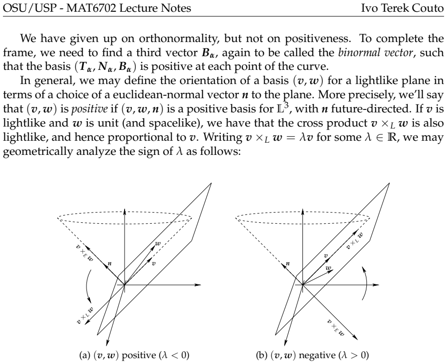
After excluding null lines, the only non-admissible biregular curves in $\mathbb{L}^3$ are lightlike curves (lightlike tangent, spacelike osculating plane) and semi-lightlike curves (spacelike tangent, lightlike osculating plane). For both classes the notes define the Cartan trihedron $(T_\alpha, N_\alpha, B_\alpha)$ with $T_\alpha=\alpha'$, $N_\alpha=\alpha''$, and $B_\alpha$ a lightlike vector completing a positive basis, and the pseudo-torsion $\wp_\alpha=-\langle N_\alpha', B_\alpha\rangle_L$. Theorem 2.18 asserts that a prescribed continuous pseudo-torsion $\wp$, a point $p_0$, and a positive initial frame satisfying the causal and orthogonality conditions determine a unique curve realizing $\wp$: in arc-photon parameter for lightlike curves, in unit speed for semi-lightlike curves. Corollary 2.19 then says that curves of either class with the same pseudo-torsion are congruent by a positive Poincaré transformation. The notes also prove the lightlike version of Lancret's theorem: a lightlike curve is a helix precisely when its pseudo-torsion is constant, and the constant-sign cases are realized by three model helices.
Load-bearing premise
The lightlike theory stands on Lemma 2.7, which asserts that a lightlike curve with nowhere-vanishing second-derivative length has an arc-photon reparametrization; the notes justify this by a first-order differential equation but do not analyze whether its solution covers the whole interval, and every later lightlike statement is made in that parameter.
Editorial extensions
If this is right
- Lightlike curves in $\mathbb{L}^3$ are locally classified by one continuous function, mirroring how Euclidean curves are classified by curvature and torsion; equal pseudo-torsion forces congruence by a positive Poincaré transformation.
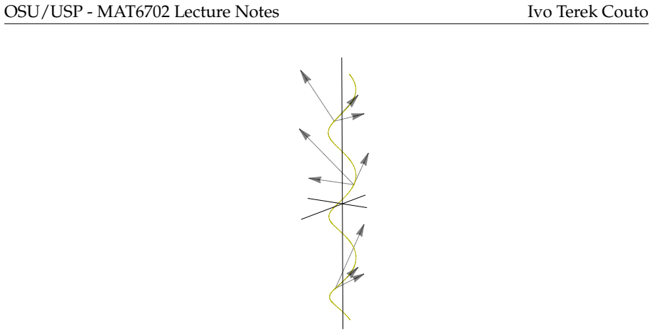
- A lightlike curve is a helix exactly when its pseudo-torsion is constant, and the sign of that constant selects one of the three model helices $\gamma_1,\gamma_2,\gamma_3$.
- Every semi-lightlike curve is contained in a lightlike plane, so its pseudo-torsion is not a measure of non-planarity; nevertheless the same initial-frame-plus-pseudo-torsion data determines it uniquely.
- For non-degenerate surfaces in $\mathbb{L}^3$, the sign of $H^2-\epsilon_M K$ decides whether the Weingarten operator is diagonalizable, giving a local answer to when principal directions exist.
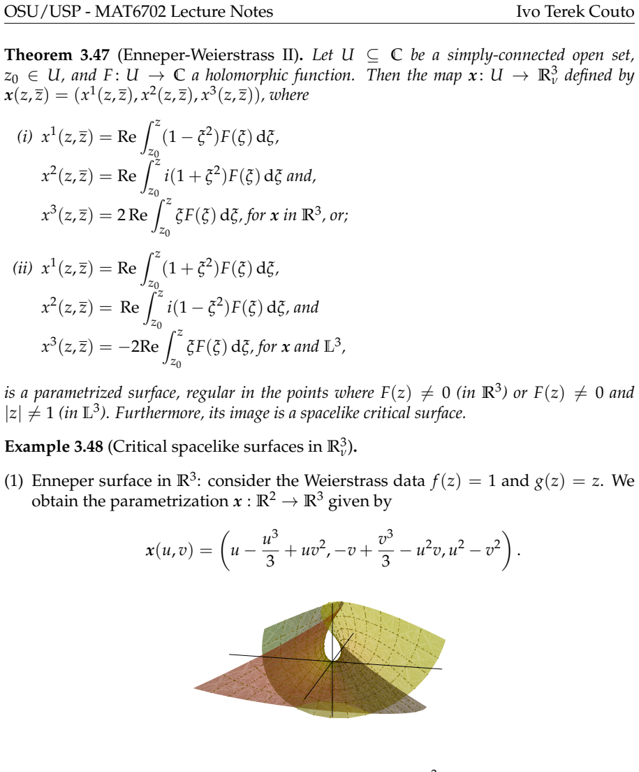
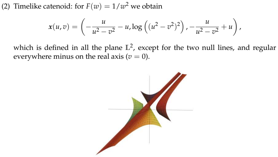
- The split-complex Weierstrass formulas produce explicit mean-curvature-zero timelike surfaces, including the timelike Enneper surface and timelike catenoid.
Reading between the lines
- Editorial extension: state Lemma 2.7 with explicit interval hypotheses; if the first-order ODE for the arc-photon reparametrization has only a local solution, then Theorems 2.13, 2.18, and 2.24 should be read as local statements, and a global version would need a separate argument.
- Editorial extension: the same frame-and-ODE strategy should extend to null curves in higher-dimensional Lorentz spaces or in other signatures, where more lightlike directions would force a larger frame; the notes do not take that step.
- Editorial extension: the omitted proof of Proposition 2.10 in the semi-lightlike case could be turned into a quantitative check: for any prescribed continuous $\wp$, solve the Theorem 2.18(ii) system and monitor $\det(T,N,B)$; a sign change would break the positivity used by the congruence statement.
Signed reviews
Editorial analysis
A structured set of objections, weighed in public.
Referee Report
Summary. The manuscript is the lecture-notes text for a mini-course given at the University of São Paulo in 2019. It contains three parts: (1) linear algebra of pseudo-Euclidean spaces, with emphasis on Lorentz-Minkowski space L3 and causal characters; (2) curve theory in L3, including admissible Frenet theory, a treatment of lightlike and semi-lightlike curves via the Cartan trihedron and pseudo-torsion, and Lancret-type classifications; (3) surface theory, covering the diagonalization problem for the Weingarten map, the local classification of constant-Gaussian-curvature surfaces, and split-complex Weierstrass representation. The main claimed contribution is Theorem 2.18, a Fundamental Theorem for lightlike and semi-lightlike curves in L3, together with the congruence corollary and the lightlike helix classification.
Significance. The notes are clearly written and the explicit computations in the examples are mostly correct: the pseudo-torsion values in Examples 2.14 and 2.16 check out, and the graph formulas of Example 3.7 are consistent with the surrounding theory. The part that goes beyond the standard admissible-curve treatment is Section 2.2, where a complete local model for lightlike and semi-lightlike curves is announced. If Theorem 2.18 and its corollaries were correctly stated and proved, the text would indeed provide a useful extension of the classical Fundamental Theorem of Curves to curves with degenerate osculating plane. However, the central theorem is false as stated, so the manuscript cannot be accepted in its current form.
major comments (2)
- [§2.2, Theorem 2.18] The hypotheses of Theorem 2.18 are incomplete. Definition 2.9 and Proposition 2.10 define the Cartan trihedron by the two conditions ⟨T,B⟩_L = -η and ⟨N,B⟩_L = -ε, so in the lightlike case one needs both ⟨T0,B0⟩_L = -1 and ⟨N0,B0⟩_L = 0, and in the semi-lightlike case one needs both ⟨N0,B0⟩_L = -1 and ⟨T0,B0⟩_L = 0. The theorem states only one of these two conditions in each case. The missing condition is not implied by positivity or by the lightlike-plane hypothesis. Concretely, in L3 with product xx′+yy′-zz′, take T0=(1,0,0), N0=(0,1,1), B0=(1,0,1), p0=0, and ♑=0. Then T0 is unit spacelike, N0 and B0 are lightlike, ⟨N0,B0⟩_L=-1, (T0,N0) is a positive basis of the lightlike plane {(a,b,b)}, and (T0,N0,B0) is positive. Thus all stated hypotheses of case (ii) hold. Yet any unit-speed semi-lightlike curve with T(0)=T0 and N(0)=N0 has binormal B(0)=(0,-1/2,1/2), not B0, because the binormal must be lightlike, Lorentz-orthogonal to T0, and satisfy ⟨N0,B(0)⟩_L=-1. Hence no such curve exists and the theorem is false as stated. A fully analogous counterexample exists for case (i), e.g. T0=(1,0,1), N0=(0,1,0), B0=(0,1,1). The theorem is repairable by adding the missing orthogonality conditions, but this is the central claim of the notes and must be corrected.
- [§2.2–§2.3, Theorems 2.18 and 2.19] The proof of case (ii) of Theorem 2.18 is left as Problem 16, and Corollary 2.19 is left as Problem 17. Since these results are the advertised fundamental theorem and its main consequence, a revised version should include a complete proof of both cases after the corrected statement. The present reliance on exercises is acceptable in lecture notes, but it is not sufficient for the central claim on which the rest of the curve theory depends.
minor comments (4)
- [§2.2, Lemma 2.7] The proof of Lemma 2.7 invokes local existence and uniqueness for the first-order ODE h′(φ)=‖α″(h(φ))‖_L^{-1/2}, but it does not justify the global assertion that h is a diffeomorphism from some open interval J onto the whole interval I. This can be settled by writing h as the inverse of s(t)=∫_{t0}^t ‖α″(u)‖_L^{1/2}du; adding this explicit construction would remove the ambiguity.
- [§2.2, Proposition 2.10] The proof of Proposition 2.10 covers only the case ε=0, η=1 and leaves the semi-lightlike case as Problem 14. Since positivity of the Cartan trihedron is used in the proof of Theorem 2.18, the corrected version should either prove the semi-lightlike case or state Proposition 2.10 with a proof for both cases.
- [§1–§3, references to [27]] Several foundational results are cited to the author's own book [27] rather than proved, including the adapted Gram-Schmidt process, the admissible Fundamental Theorem of Curves, some surface computations, and the classification of split-holomorphic functions. If the notes are intended to be self-contained, those results should be stated explicitly with clear references; if not, a short remark on the division of labor between the notes and [27] would help the reader.
- [§3.1, Example 3.7(2)] The sign of the Gauss map for the hyperbolic plane should be specified: with N(p)=p the position map gives scalar mean curvature H=-1, whereas the stated value H=1 corresponds to N(p)=-p. Adding one sentence clarifying the choice of Gauss map would avoid confusion.
Circularity Check
No load-bearing circularity: Theorem 2.18 and the Cartan-frame theory are proved in the text; self-citations to the author's own book [27] supply standard background; the substantive flaw (missing Gram hypotheses in Theorem 2.18) is a correctness gap, not circularity.
full rationale
The central claim, Theorem 2.18 (Fundamental Theorem for lightlike and semi-lightlike curves), is derived in-text rather than imported: the Cartan system (Theorem 2.13) is proved from Definition 2.9 and the expansion Lemma 2.11; Theorem 2.18 is then proved by a linear IVP in R^9, with the constraint algebra preserved by the companion IVP in R^6 whose initial vector a(φ0) = (0,1,0,0,-1,0) is a constant solution. The prescribed pseudo-torsion is not folded into the conclusion by definition: the curve is constructed as α(φ) = p0 + ∫ T, so Tα = T and Nα = N by construction, and ♑α = ♑ is recovered in the last step by differentiating N and comparing with the second Cartan equation — the standard existence argument of a Fundamental Theorem, where the data (♑, frame) are genuinely smaller than the output (curve). Corollaries 2.19, 2.23 and 2.24 rest on this in-text argument. There is no data fitting, no renamed known result presented as new, and no uniqueness theorem imported from the author's prior work. The repeated citations to [27] (Terek–Lymberopoulos, a published SBM volume whose first author is the present author) cover standard background — the adapted Gram–Schmidt details (Sec. 1.1), the admissible-curve Fundamental Theorem 2.6 (Sec. 2.1), the surface-coefficient computations (Sec. 3.1), and the classification of split-holomorphic functions (Extra #2). These are independently grounded in the classical references the notes also cite ([13], [18], [19], [20], [23]), so none is load-bearing circularity under the stated rules; the most substantive delegation, Theorem 2.6, is the classical result whose R3 prototype the notes sketch, and it underlies only the standard admissible half of the notes. The genuine problems in the paper are omissions and a correctness error, which I am deliberately not scoring as circularity: Lemma 2.7 asserts existence and uniqueness of the arc-photon ODE without domain analysis; Proposition 2.10's semi-lightlike case and Theorem 2.18 case (ii) are left to Problem 14 and Problem 16; and Theorem 2.18 omits the second Cartan Gram condition — case (i) also needs ⟨N0,B0⟩ = 0 and case (ii) also needs ⟨T0,B0⟩ = 0 — while the proof's initial vector silently assumes them, so the theorem is false as stated (e.g., case (ii) with T0=(1,0,0), N0=(0,1,1), B0=(1,0,1), ♑=0 satisfies the stated hypotheses but any unit-speed curve has B = (0,-1/2,1/2) ≠ B0).
Assumptions & free parameters
assumptions (6)
- standard math Existence and uniqueness of solutions of the linear R9 Frenet-type initial value problem (Theorem 2.18)
- standard math Arc-photon reparametrization ODE h' = ||α''(h)||_L^{-1/2} has a unique solution (Lemma 2.7)
- standard math Milnor's sharpened spectral theorem for self-adjoint operators with dim V >= 3
- standard math Alexandrov-Zeeman theorem (Theorem 1.29)
- standard math Conjugacy classification of O+↑_1(3,R) (Theorem 1.22)
- standard math Standard geodesic facts: existence of unit speed geodesics, Fermi chart regularity
Cite this review
Pith. "Pith review of Topics in Lorentz Geometry." pith.science (2026). https://pith.science/paper/L4YSXZ7B
@misc{pith2026190801710,
  author       = {Pith},
  title        = {Pith review of: Topics in Lorentz Geometry},
  year         = {2026},
  howpublished = {\url{https://pith.science/paper/L4YSXZ7B}},
  note         = {Machine review of arXiv:1908.01710}
}
abstract
Lecture notes from the mini-course "Topics in Lorentz Geometry" taught at the University of S\~{a}o Paulo, in March/2019. The text has three parts: (i) an overall view of linear algebra in the pseudo-Euclidean space $\mathbb{R}^n_\nu$, with focus on Lorentz-Minkowski space and its role in Physics; (ii) a version of the Fundamental Theorem of Curves in 3-dimensional Lorentz-Minkowski space, with adaptations to curves with degenerate osculating plane; (iii) the problem of the diagonalization of the Weingarten map for timelike surfaces, local classification of surfaces with constant Gaussian curvature $K$ and Weierstrass' representation formula in Lorentz-Minkowski space (using split-complex algebra). V2: added references.
Figures

Figures from the paper (20 more)









Reference graph
Works this paper leans on
-
[27]
Terek, I.; Lymberopoulos, A.; Introdução à Geometria Lorentziana: Curvas e Superfí- cies, SBM (Universitary Texts Collection, volume 21), 2018. Page 74 OSU/USP - MAT6702 Lecture Notes Ivo Terek Couto Index ν-orthogonality, 6 Admissible curve, 23 Anti-de Sitter space, 49 Arc-photon reparametrization, 25 Biregular curve, 22 B-scroll (associated to a lightli...
work page 2018
-
[18]
Konderak, J.; A Weierstrass Representation Theorem for Lorentz Surfaces , Complex Variables 50 (no. 5, pp.319-332), 2005
work page 2005
-
[19]
López, R., Differential Geometry of Curves and Surfaces in Lorentz–Minkowski space, eprint arXiv:0810.3351, https://arxiv.org/pdf/0810.3351, 2008
arXiv 2008
-
[20]
Magid, M.; Minimal Timelike Surfaces via the Split-Complex Numbers, Proceedings of PADGE 2012, Shaker-Verlag, Aachen, 2013
work page 2012
-
[1]
Alexandrov, D., A contribution to chronogeometry, Canadian J. Math. 19, pp. 1119- 1128, 1967
work page 1967
-
[2]
Alias, L.; Chaves, R. M. B.; Mira, P .;Bjorling roblem for maximal surfaces in Lorentz- Minkowski space, Math. Proc. Camb. Phil. Soc. (no. 134, pp. 289-316), 2003
work page 2003
-
[3]
Chaves, R. M. B.; Dussan, M. P .; Magid, M.;Bjorling Problem for timelike surfaces in the Lorentz-Minkowski space, Journal of Mathematical Analysis and Applciations (377, no. 2, pp; 481-494), 2011
work page 2011
-
[4]
Anciaux, H., Minimal Submanifolds in Pseudo-Riemannian Geometry, World Scien- tific, 2011
work page 2011
Show all 27 references
-
[5]
Antonuccio, F., Semi–Complex Analysis & Mathematical Physics (Corrected Version), eprint arXiv:gr-qc/9311032, 1993, https://arxiv.org/pdf/gr-qc/9311032. pdf
1993 arXiv
-
[6]
K.; Ehrlich, P
Beem, J. K.; Ehrlich, P . E.; Easley, K. L., Global Lorentzian Geometry , CRC Press, 1996
1996
-
[7]
Catoni et al., Geometry of Minkowski Spacetime , Springer-Verlag (Springer Briefs in Physics), 2011
2011
-
[8]
Y.; Pseudo-Riemannian Geometry, δ-invariants and Applications, World Sci- entific, 2011
Chen, B. Y.; Pseudo-Riemannian Geometry, δ-invariants and Applications, World Sci- entific, 2011
2011
-
[9]
P ., Geometria Diferencial de Curvas e Superfícies, SBM (Universitary Texts Collection, volume 04), 2014
do Carmo, M. P ., Geometria Diferencial de Curvas e Superfícies, SBM (Universitary Texts Collection, volume 04), 2014
2014
-
[10]
P .; Franco Filho, A
Dussan, M. P .; Franco Filho, A. P .; Magid, M.; The Bjorling Problem for timelike minimal surfaces in R4 1, Annali di Matematica Pura ed Applicata (pp. 1-19), 2016
2016
-
[11]
P .; Magid, M.; Bjorling Problem for timelike surfaces in R4 2, Journal of Geometry and Physics (no
Dussan, M. P .; Magid, M.; Bjorling Problem for timelike surfaces in R4 2, Journal of Geometry and Physics (no. 73, pp. 187-199), 2013
2013
-
[12]
M.; Margulis, G
Goldman, W. M.; Margulis, G. A., Flat Lorentz 3-manifolds and cocompact Fuchsian groups. Crystallographic groups and their generalizations (Kortrijk, 1999) Contempo- rary Mathematics 262, pp. 135—145, 2000
1999
-
[13]
H., Linear Algebra, Springer-Verlag, 1975
Greub, W. H., Linear Algebra, Springer-Verlag, 1975
1975
-
[14]
Hawking, S., Ellis, G.; The Large Scale Structure of Spacetime , Cambridge Mono- graphs on Mathematical Physics, 1973
1973
-
[15]
23–28, 2011
Hitzer, E., Non-constant bounded holomorphic functions of hyperbolic numbers – Can- didates for hyperbolic activation functions , Proccedings of the First SICE Sympo- sium on Computational Intelligence, pp. 23–28, 2011. Page 73 OSU/USP - MAT6702 Lecture Notes Ivo Terek Couto
2011
-
[16]
4–14, 2014
Kosheleva, O.; Kreinovich, V ., Observable Causality Implies Lorentz Group: Alexandrov–Zeeman–Type Theorem for Space–Time Regions , Mathematical Struc- tures and Modeling 30, pp. 4–14, 2014
2014
-
[17]
Kobayashi, O., Maximal Surfaces in the 3-Dimensional Minkowski Space L3, Tokyo J. of Math. Volume 06, pp. 297–309, 1983
1983
-
[21]
L., Spacetime and Singularities, An Introduction , Cambridge University Press, 1988
Naber, G. L., Spacetime and Singularities, An Introduction , Cambridge University Press, 1988
1988
-
[22]
L., The Geometry of Minkowski Spacetime: An Introduction to the Mathe- matics of the Special Theory of Relativity , Springer–Verlag (Applied Mathematical Sciences 92), 1992
Naber, G. L., The Geometry of Minkowski Spacetime: An Introduction to the Mathe- matics of the Special Theory of Relativity , Springer–Verlag (Applied Mathematical Sciences 92), 1992
1992
-
[23]
O’Neill, B., Semi-Riemannian Geometry with Applications to Relativity , Academic Press, 1983
1983
-
[24]
Osserman, R., A Survey of Minimal Surfaces, Dover, 1986
1986
-
[25]
Penrose, R., Techniques of Differential Topology in Relativity, AMS Coloquium Pub- lications (SIAM, Philadelphia), 1972
1972
-
[26]
Tenenblat, K., Introdução à Geometria Diferencial, Edgard Blücher, 2008
2008
Reviewed August 14, 2026 · model on record in the stance chip above.
Discussion (0). Continue with ORCID to comment.