REVIEW 3 major objections 4 minor 51 references
Plateau de Bure High-z Blue-Sequence Survey 2 (PHIBSS2): Search for Secondary Sources, CO Luminosity Functions in the Field, and the Evolution of Molecular Gas Density through Cosmic Time
T0 review · 3 major / 4 minor · reviewed 2026-08-14 · deepseek-v4-flash
Pith's one-line read A blind search inside targeted galaxy data cubes reconstructs field carbon-monoxide luminosity functions.
desk verdict A careful, genuinely useful mining of targeted PHIBSS2 cubes for serendipitous CO sources, with a catalog and luminosity functions that support the method but do not yet nail the quantitative agreement with blind surveys. read the letter →
The pith
A machine-rendered reading of the paper's core claim, the machinery that carries it, and where it could break.
The reading
What carries the argument
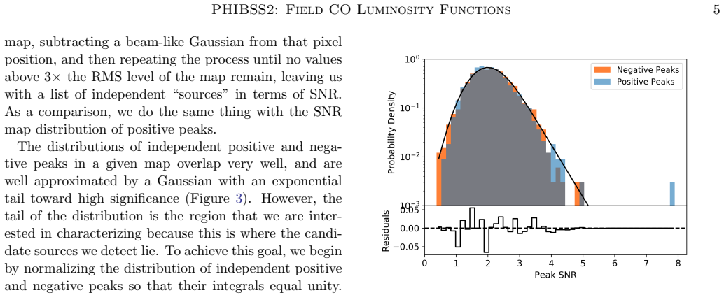
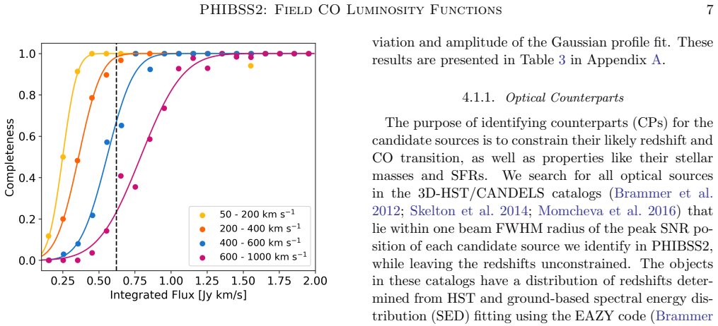
The central mechanism is a blind matched-filter line search over each spectral cube. Every cube is Hanning-smoothed and decimated to five velocity resolutions; the peak of each pixel spectrum is divided by a polynomial model of the local noise to form signal-to-noise maps. The noise side is calibrated empirically from the distribution of negative peaks, fit by an exponentially modified Gaussian, and each candidate is assigned a reliability $R = 1 - N_{\rm expected}/N_{\rm beams}$. Completeness comes from injecting 2500 artificial beam-shaped Gaussian sources per cube. The luminosity function estimator $$\Phi(\log L_i) = \frac{1}{V}\sum_{j=1}^{N_i} \frac{R_j}{C_j} P_{a,j} P_{z,j}$$ then converts the weighted candidate counts into comoving space densities, dividing by the volume $V$ sampled by each transition, upweighting by completeness $C_j$, and downweighting by reliability, optical-counterpart association, and transition/redshift probability.
What would settle it
Spectroscopically determine the redshifts of all 67 CO candidates, especially the 24 without optical counterparts; if a substantial fraction turn out to be real sources at transitions or redshifts outside the assumed CO(1-0) through CO(6-5) ladder, the luminosity functions and gas density points would move off the blind-survey curves.
Extended reading notes
Core claim
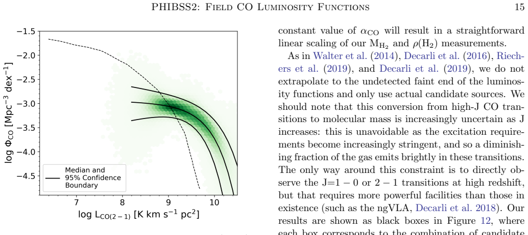
The paper's claim is that serendipitous CO sources found inside targeted observations are field galaxies rather than satellites of the primary targets, and that their counts can be turned into measurements of the CO luminosity function and the cosmic molecular gas density. From 67 candidate sources in 110 data cubes, with per-source reliability, completeness, counterpart-association, and redshift-probability weighting, the paper constructs CO(2-1), CO(3-2), CO(4-3), CO(5-4), and CO(6-5) luminosity functions at median redshifts from about 0.7 to 3.6. It reports that these agree with earlier blind-search constraints, and interprets the agreement as evidence that the serendipitous sample is not biased toward the primary targets and that combining many independent lines of sight reduces cosmic variance. Because sources without optical counterparts are excluded, the luminosity functions are lower limits.
Load-bearing premise
Each serendipitous source gets its redshift by being matched to an optical galaxy within one telescope beam and by assuming its detected line is one of six carbon monoxide rotational transitions; the 36 percent of sources with no optical match are excluded, so the measured luminosity functions are lower limits.
Editorial extensions
If this is right
- Existing targeted CO surveys can be re-analyzed with the same blind-search pipeline to produce field CO luminosity functions, adding deep-field science without new observing time.
- The 67-source catalog presents a CO-selected sample of galaxies with measured fluxes, line widths, reliabilities, and counterpart associations, available for follow-up study of gas-rich galaxies outside the original target selection.
- Combining many independent sightlines keeps cosmic variance at roughly 13-18 percent, so serendipitous surveys can be competitive with contiguous deep fields for a small fraction of the observing time.
- The CO luminosity functions at redshifts of about 0.7 to 3.6 tighten constraints on the evolution of the cosmic molecular gas density, including an apparent excess of high-J CO-bright galaxies over current theoretical predictions.
Reading between the lines
- Inference: If the same pipeline were applied to other large targeted interferometric surveys, the serendipitous sample could grow to hundreds of sources, allowing finer luminosity-binning and a fainter reach than this 110-cube dataset.
- Inference: Because the 36 percent of sources without optical counterparts are dropped, the true molecular gas density may be higher than the reported lower limits, especially if those sources are dust-obscured galaxies missed by rest-optical catalogs.
- Inference: The paper's mass-SFR comparison implies that optical-to-8-micron SED fits underestimate star formation in CO-selected galaxies; a testable consequence is that adding far-infrared photometry should bring SED-inferred and CO-inferred gas masses into agreement for most counterparts.
- Inference: A redshift-space cross-correlation of the serendipitous sources with the primary targets would give a quantitative check on the no-clustering assumption; a signal at $\Delta z \lesssim 0.1$ would require adding a clustering bias term to the luminosity function estimator.
Signed reviews
Editorial analysis
A structured set of objections, weighed in public.
Referee Report
Summary. This paper reports a blind search for serendipitous CO line emitters in the 110 targeted PHIBSS2 data cubes of z~1-2 main-sequence galaxies. The authors develop a matched-filter line search with per-cube noise modeling, estimate candidate reliability from the statistics of negative noise peaks, and characterize completeness by injecting 2500 artificial sources per cube. They obtain a catalog of 67 candidates, find tentative 3D-HST/CANDELS counterparts for 43 (64%), assign CO transitions and redshifts via photometric-redshift posteriors, and construct CO(2-1) through CO(6-5) luminosity functions over z~0.5-5 plus a molecular gas mass density evolution measurement. The main astrophysical claim is that these serendipitous-source measurements agree well with previous blind-survey results (COLDz, ASPECS, PdBI HDF-N), demonstrating the utility of targeted observations for field CO luminosity function measurements.
Significance. If the central claim holds, the paper provides a valuable new route to field CO luminosity functions and gas density evolution by repurposing existing targeted observations, and the catalog of 67 candidates is a useful community resource. The methodological care is explicit: false-positive probabilities come from a parametric fit to negative noise peaks, completeness is measured via injection-recovery simulations with beam and primary-beam corrections, and volumes account for primary-beam attenuation. The multi-sightline approach also reduces cosmic variance relative to contiguous deep fields, as quantified with the Driver & Robotham (2010) formalism. These strengths are real and should be credited. However, the luminosity functions depend on photometric-redshift-based transition identification for 43 sources, with 24 sources excluded as unresolved without counterparts, so the quantitative agreement with earlier work is contingent on the reliability of those identifications.
major comments (3)
- [§4.3, Eq. (9), and §4.3.1] The reported error bars in Figure 9 and Table 5 are Poissonian only (Gehrels 1986) and do not include uncertainties in the weights R, C, Pa, and Pz. Because the luminosity functions are weighted sums over these quantities, the systematic uncertainties—especially in the completeness correction C and the redshift probability Pz—can be comparable to or larger than the Poisson errors, particularly in the faintest bins. The 'very good agreement' with COLDz and ASPECS claimed in the abstract and §5 depends on these error bars. I recommend propagating all uncertainties (e.g., through a Monte Carlo or bootstrap over the noise-model fits, completeness fits, counterpart association, and redshift posteriors) or, at minimum, presenting the luminosity functions with an explicit systematic-error band and adjusting the agreement claim in the abstract accordingly.
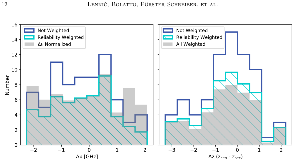
- [§4.1.1 and Table 4] The redshift/transition assignment for each serendipitous source relies on matching a single observed line frequency to CO(1-0) through CO(6-5) using the EAZY photometric-redshift posterior. For several sources (e.g., xc55-3, gn010-6, gn018-2, eg012-1) the posterior permits multiple transitions, and the adopted Pz is described qualitatively rather than defined precisely. The derivation should state the exact formula used for Pz and demonstrate that the resulting luminosity functions are insensitive to alternative, equally plausible posterior-weighting schemes, or show how the LFs change when restricted to sources with spectroscopic/grism redshifts. This is directly relevant to the CO(2-1) and CO(3-2) bins compared to COLDz and ASPECS in §5.1.1.
- [§4.1.1, Figure 6, and §5.1.1] The large (1-2 order-of-magnitude) offset between CO-based molecular gas masses and SFR-based masses for most matched sources is attributed to obscured star formation, but the same signature would be produced by a non-negligible fraction of misassociated counterparts or incorrectly assigned transitions. The paper uses the agreement of the derived luminosity functions with blind-survey results as evidence that misidentification is not the dominant effect, which is circular because the luminosity functions themselves are built from these identifications. An independent validation would strengthen the paper: for example, a comparison of the LF after removing sources with low R × Pa, a stacking analysis to confirm candidate lines at counterpart positions, or a demonstration that the subset with secure (spectroscopic/grism) redshifts alone reproduces the LF.
minor comments (4)
- [Table 4, EGS rows] The coordinate for eg012-1 is given as '2d51m9.70s', presumably '52d51m9.70s'; please correct the typo.
- [§3.1.2, last paragraph] The statement that simulating sources 'at the edges of pixels and at the centers of pixels' has negligible impact would be clearer if the text distinguished between pixel edges and primary-beam edges, since the primary-beam sensitivity drop-off is treated separately in the volume calculation.
- [Figure 9 and Table 5] Because the bins are 0.5 dex wide and stepped at 0.1 dex, adjacent points are strongly correlated; the text notes that every 5th bin is independent, but the caption should also state this so that readers do not treat adjacent points as independent.
- [Abstract and §1] '45 out of the 110 data cubes showing sources' followed by a catalog of 67 candidates is clear, but the sentence would benefit from explicitly stating that some cubes contain multiple candidates.
Circularity Check
No significant circularity: the CO luminosity functions are direct weighted sums of measured candidates, and the external comparisons serve as benchmarks rather than fit inputs.
full rationale
The paper's central claim is a measurement, not a fitted prediction. Equation 9 builds each luminosity function as a sum over candidate sources of R_j/C_j times Pa,j and Pz,j, where R_j is the reliability from negative-noise statistics, C_j is the completeness from injected-source simulations, and Pa,j and Pz,j come from matching to 3D-HST/CANDELS counterparts and EAZY redshift posteriors. None of these weights is tuned to match the COLDz, ASPECS, or model luminosity functions shown in Figure 9; the comparisons to Walter et al. (2014), Decarli et al. (2016, 2019), and Riechers et al. (2019) are made after the fact. The conversion from high-J CO to CO(1-0) and molecular gas mass uses literature values (Daddi et al. 2015 r_J1 ratios and alpha_CO = 3.6) with stated assumptions, and the paper explicitly notes that varying alpha_CO only rescales the gas densities linearly. The only self-referential element is the use of the Tacconi et al. (2018) depletion-time scaling in the Figure 6 cross-check, but that comparison is a consistency diagnostic and is not an input to the luminosity functions or the gas-density evolution. The paper also states clearly that excluding the 36% of candidates without optical counterparts makes the luminosity functions lower limits; this is a completeness caveat, not a circular step. The agreement with blind surveys is therefore a genuine external benchmark, and any concern about misidentified counterparts or unquantified systematics belongs under systematic uncertainty rather than circularity.
Assumptions & free parameters
free parameters (3)
- Completeness correction fit parameters (mu, sigma per cube) =
Fitted per cube via cumulative Gaussian to injection recovery fractions
- Exponentially modified Gaussian noise parameters (mu, sigma, lambda) for reliability =
Fitted per cube to the negative-peak SNR distribution
- RMS polynomial order =
7
assumptions (6)
- domain assumption Detected serendipitous lines are CO rotational transitions from J_upper=1 to 6 at the redshift of a tentative optical counterpart.
- domain assumption The noise distribution in each cube is symmetric, so negative-peak statistics characterize false positives.
- domain assumption Injected Gaussian sources recover the search completeness as a function of integrated flux.
- domain assumption Adopted conversion factors alpha_CO = 3.6 and r_J1 ratios from Daddi et al. (2015) apply to the field sources.
- standard math Lambda-CDM cosmology with H0 = 70, Omega_m = 0.3, Omega_Lambda = 0.7.
- domain assumption The 3D-HST/CANDELS photometric redshifts and EAZY posteriors are reliable enough to constrain CO transition probabilities.
Cite this review
Pith. "Pith review of Plateau de Bure High-z Blue-Sequence Survey 2 (PHIBSS2): Search for Secondary Sources, CO Luminosity Functions in the Field, and the Evolution of Molecular Gas Density through Cosmic Time." pith.science (2026). https://pith.science/paper/A2WFV7BA
@misc{pith2026190801791,
  author       = {Pith},
  title        = {Pith review of: Plateau de Bure High-z Blue-Sequence Survey 2 (PHIBSS2): Search for Secondary Sources, CO Luminosity Functions in the Field, and the Evolution of Molecular Gas Density through Cosmic Time},
  year         = {2026},
  howpublished = {\url{https://pith.science/paper/A2WFV7BA}},
  note         = {Machine review of arXiv:1908.01791}
}
read the original abstract
We report on the results of a search for serendipitous sources in CO emission in 110 cubes targeting CO(2-1), CO(3-2), and CO(6-5) at z ~ 1-2 from the second Plateau de Bure High-z Blue-Sequence Survey (PHIBSS2). The PHIBSS2 observations were part of a 4-year legacy program at the IRAM Plateau de Bure Interferometer aimed at studying early galaxy evolution from the perspective of molecular gas reservoirs. We present a catalog of 67 candidate secondary sources from this search, with 45 out of the 110 data cubes showing sources in addition to the primary target that appear to be field detections, unrelated to the central sources. This catalog includes the redshifts, line widths, fluxes, as well as an estimation of their reliability based on their false positive probability. We perform a search in the 3D-HST/CANDELS catalogs for the secondary CO detections and tentatively find that ~64% of these have optical counterparts, which we use to constrain their redshifts. Finally, we use our catalog of candidate CO detections to derive the CO(2-1), CO(3-2), CO(4-3), CO(5-4), and CO(6-5) luminosity functions over a range of redshifts, as well as the molecular gas mass density evolution. Despite the different methodology, these results are in very good agreement with previous observational constraints derived from blind searches in deep fields. They provide an example of the type of "deep field" science that can be carried out with targeted observations.
Figures


Figures from the paper (11 more)






Reference graph
Works this paper leans on
-
[1]
P., Tollerud, E
Astropy Collaboration, Robitaille, T. P., Tollerud, E. J., et al. 2013, A&A, 558, A33
2013
-
[2]
Frayer, D. T. 2002, PhR, 369, 111
work page 2002
-
[3]
D., Wolfire, M., & Leroy, A
Bolatto, A. D., Wolfire, M., & Leroy, A. K. 2013, ARA&A, 51, 207
2013
-
[4]
D., Warren, S
Bolatto, A. D., Warren, S. R., Leroy, A. K., et al. 2015, ApJ, 809, 175
2015
-
[5]
B., van Dokkum, P
Brammer, G. B., van Dokkum, P. G., & Coppi, P. 2008, ApJ, 686, 1503
2008
-
[6]
B., van Dokkum, P
Brammer, G. B., van Dokkum, P. G., Franx, M., et al. 2012, ApJS, 200, 13
2012
- [7]
-
[8]
Carleton, T., Cooper, M. C., Bolatto, A. D., et al. 2017, MNRAS, 467, 4886
work page 2017
Show all 51 references
-
[9]
M., Narayanan, D., & Cooray, A
Casey, C. M., Narayanan, D., & Cooray, A. 2014, PhR, 541, 45
2014
-
[10]
2010, ApJ, 713, 686
Daddi, E., Bournaud, F., Walter, F., et al. 2010, ApJ, 713, 686
2010
-
[11]
2015, A&A, 577, A46
Daddi, E., Dannerbauer, H., Liu, D., et al. 2015, A&A, 577, A46
2015
-
[12]
2014, ApJ, 782, 78
Decarli, R., Walter, F., Carilli, C., et al. 2014, ApJ, 782, 78
2014
-
[13]
2016, ApJ, 833, 69
Decarli, R., Walter, F., Aravena, M., et al. 2016, ApJ, 833, 69
2016
-
[14]
2018, in Astronomical Society of the Pacific Conference Series, Vol
Decarli, R., Carilli, C., Casey, C., et al. 2018, in Astronomical Society of the Pacific Conference Series, Vol. 517, Science with a Next Generation Very Large Array, ed. E. Murphy, 565
2018
-
[15]
2019, ApJ, 882, 138
Decarli, R., Walter, F., G´ onzalez-L´ opez, J., et al. 2019, ApJ, 882, 138
2019
-
[16]
P., & Robotham, A
Driver, S. P., & Robotham, A. S. G. 2010, MNRAS, 407, 2131
2010
-
[17]
J., et al
Freundlich, J., Combes, F., Tacconi, L. J., et al. 2019, A&A, 622, A105
2019
-
[18]
1986, ApJ, 303, 336
Gehrels, N. 1986, ApJ, 303, 336
1986
-
[19]
J., Gracia-Carpio, J., et al
Genzel, R., Tacconi, L. J., Gracia-Carpio, J., et al. 2010, MNRAS, 407, 2091
2010
-
[20]
J., Lutz, D., et al
Genzel, R., Tacconi, L. J., Lutz, D., et al. 2015, ApJ, 800, 20 Gonz´ alez-L´ opez, J., Decarli, R., Pavesi, R., et al. 2019, ApJ, 882, 139
2015
-
[21]
R., Bertoldi, F., Smail, I., et al
Greve, T. R., Bertoldi, F., Smail, I., et al. 2005, MNRAS, 359, 1165
2005
-
[22]
1992, A&A, 262, 624
Guilloteau, S., Delannoy, J., Downes, D., et al. 1992, A&A, 262, 624
1992
-
[23]
Hunter, J. D. 2007, Computing in Science & Engineering, 9, 90
2007
-
[24]
M., & Gunn, J
Kent, S. M., & Gunn, J. E. 1982, AJ, 87, 945
1982
-
[25]
M., Dunkley, J., et al
Komatsu, E., Smith, K. M., Dunkley, J., et al. 2011, ApJS, 192, 18
2011
-
[26]
Lagos, C. D. P., Baugh, C. M., Lacey, C. G., et al. 2011, MNRAS, 418, 1649
2011
-
[27]
Lagos, C. d. P., Bayet, E., Baugh, C. M., et al. 2012, MNRAS, 426, 2142
2012
-
[28]
2014, ARA&A, 52, 415
Madau, P., & Dickinson, M. 2014, ARA&A, 52, 415
2014
-
[29]
G., Brammer, G
Momcheva, I. G., Brammer, G. B., van Dokkum, P. G., et al. 2016, ApJS, 225, 27
2016
-
[30]
2009, ApJ, 702, 1321
Obreschkow, D., Heywood, I., Kl¨ ockner, H.-R., & Rawlings, S. 2009, ApJ, 702, 1321
2009
-
[31]
2000, A&AS, 143, 23
Ochsenbein, F., Bauer, P., & Marcout, J. 2000, A&AS, 143, 23
2000
-
[32]
Oliphant, T. E. 2015, A guide to NumPy, 2nd edn. (7290 Investment Drive # B, North Charleston, SC, United States: CreateSpace Independent Publishing Platform)
2015
-
[33]
E., Riechers, D
Pavesi, R., Sharon, C. E., Riechers, D. A., et al. 2018, ApJ, 864, 49 P´ erez, F., & Granger, B. E. 2007, Computing in Science and Engineering, 9, 21
2018
-
[34]
2016, MNRAS, 461, 93
Popping, G., van Kampen, E., Decarli, R., et al. 2016, MNRAS, 461, 93
2016
-
[35]
S., et al
Popping, G., Pillepich, A., Somerville, R. S., et al. 2019, ApJ, 882, 137
2019
-
[36]
M., Sip˝ ocz, B
Price-Whelan, A. M., Sip˝ ocz, B. M., G¨ unther, H. M., et al. 2018, AJ, 156, 123
2018
-
[37]
A., Pavesi, R., Sharon, C
Riechers, D. A., Pavesi, R., Sharon, C. E., et al. 2019, ApJ, 872, 7
2019
-
[38]
2012, APLpy: Astronomical Plotting Library in Python, Astrophysics Source Code Library, , , ascl:1208.017
Robitaille, T., & Bressert, E. 2012, APLpy: Astronomical Plotting Library in Python, Astrophysics Source Code Library, , , ascl:1208.017
2012
-
[39]
C., Burstein, D., Ford, Jr., W
Rubin, V. C., Burstein, D., Ford, Jr., W. K., & Thonnard, N. 1985, ApJ, 289, 81
1985
-
[40]
1976, ApJ, 203, 297
Schechter, P. 1976, ApJ, 203, 297
1976
-
[41]
2014, IRAM Annu
Schuster, K.-F. 2014, IRAM Annu. Rep. https://www.iram- institute.org/medias/uploads/IRAM 2014.pdf
2014
-
[42]
E., Whitaker, K
Skelton, R. E., Whitaker, K. E., Momcheva, I. G., et al. 2014, ApJS, 214, 24
2014
-
[43]
M., Downes, D., Radford, S
Solomon, P. M., Downes, D., Radford, S. J. E., & Barrett, J. W. 1997, ApJ, 478, 144
1997
-
[44]
J., Genzel, R., Neri, R., et al
Tacconi, L. J., Genzel, R., Neri, R., et al. 2010, Nature, 463, 781
2010
-
[45]
J., Neri, R., Genzel, R., et al
Tacconi, L. J., Neri, R., Genzel, R., et al. 2013, ApJ, 768, 74
2013
-
[46]
J., Genzel, R., Saintonge, A., et al
Tacconi, L. J., Genzel, R., Saintonge, A., et al. 2018, ApJ, 853, 179 PHIBSS2: Field CO Luminosity Functions 29
2018
-
[47]
2016, MNRAS, 456, L40
Zamorani, G. 2016, MNRAS, 456, L40
2016
-
[48]
2014, ApJ, 782, 79
Walter, F., Decarli, R., Sargent, M., et al. 2014, ApJ, 782, 79
2014
-
[49]
2016, ApJ, 833, 67
Walter, F., Decarli, R., Aravena, M., et al. 2016, ApJ, 833, 67
2016
-
[50]
E., Pope, A., Cybulski, R., et al
Whitaker, K. E., Pope, A., Cybulski, R., et al. 2017, ApJ, 850, 208
2017
-
[51]
M., Lutz, D., et al
Wuyts, S., F¨ orster Schreiber, N. M., Lutz, D., et al. 2011, ApJ, 738, 106
2011
Reviewed August 14, 2026 · model on record in the stance chip above.
Discussion (0). Continue with ORCID to comment.