Safe Control Algorithms Using Energy Functions: A Unified Framework, Benchmark, and New Directions

Changliu Liu; Tianhao Wei

REVIEW 3 major objections 5 minor 19 references

Safe Control Algorithms Using Energy Functions: A Unified Framework, Benchmark, and New Directions

T0 review · 3 major / 5 minor · reviewed 2026-08-14 · deepseek-v4-flash

Challenge this review Re-run · record.json Download PDF Read on arXiv ↗ Review JSON

Pith's one-line read A single control law unifies four safe-control methods, and the paper's sublevel safe set variant wins most benchmark tests.

desk verdict A genuinely useful unification and benchmark, undermined by a framework whose core assumption excludes the velocity-dependent safety index the experiments actually use. read the letter →

arxiv 1908.01883 v2 pith:FSIUG7VZ submitted 2019-08-05 eess.SY cs.SY

Tianhao Wei , Changliu Liu This is my paper · ORCID

classification eess.SYcs.SY

keywords safecontrolenergyfunctionbarrierfunctionssetalgorithmpotentialfieldmethodslidingmodesublevelhuman-robotinteractionbenchmark

verification ladder T0 review T1 audit T2 compute T3 formal

The pith

A machine-rendered reading of the paper's core claim, the machinery that carries it, and where it could break.

The reading

This paper tries to establish that four common safe-control recipes—potential field method, sliding mode algorithm, safe set algorithm, and barrier function method—are all one algorithm: each steers the state by decreasing a scalar energy function along the direction of its control sensitivity. The unification rests on a perpendicular decomposition of the control input into a safety component along the Lie derivative and an efficiency component orthogonal to it. The paper then derives a new controller, the sublevel safe set algorithm, which combines the rare but decisive corrections of the safe set algorithm with the frequent but gentle corrections of the barrier function method. In the paper's benchmark across four robot models and interaction modes, this new method reports the best safety-efficiency trade-off on the vast majority of tests. If correct, the framework gives a common vocabulary for comparing safe controllers and a principled way to design new ones.

What carries the argument

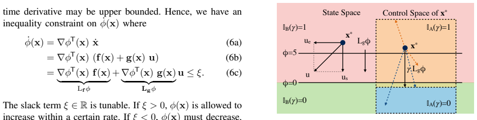
The load-bearing object is the orthogonal decomposition of the control input with respect to the Lie derivative $L_g\varphi$, where $\varphi$ is the scalar energy function measuring safety. Because $\dot\varphi = L_f\varphi + L_g\varphi\, u$, only the component of $u$ parallel to $L_g\varphi$ changes the energy, so every safety constraint becomes a half-space inequality on that component. This reduces each algorithm to a choice of the scalar gain $\alpha$ and the slack term $\xi$, which lets PFM, SMA, SSA, BFM, and the proposed SSS be compared by just two numbers rather than by their original problem formulations.

What would settle it

Log the states from the benchmark and, at each logged state, recompute the control from the safe set and barrier function optimization problems and compare it with the unified formula $\alpha L_g\varphi^T + u_0^e$ using $\varphi = d_{\min}^2 - d^2 - k\dot d$; the formulas will disagree whenever $\dot d$ is influenced by the obstacle's velocity, which would show the unification theorem is not directly exercised by the benchmark.

Watch

Extended reading notes

Core claim

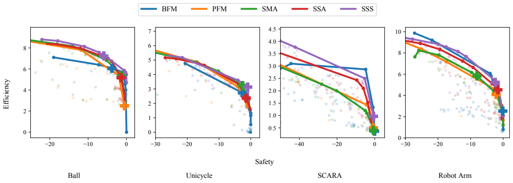
The central claim is that PFM, SMA, SSA, and BFM are all instances of a single energy-function-based control law: the safety component of the input is $\alpha L_g\varphi^T$, the efficiency component is the reference control projected orthogonal to $L_g\varphi$, and in all four methods $\beta = 0$ (Theorem 1). The paper gives explicit formulas for the scalar gain $\alpha$ in each method: PFM and SMA add a constant-scale correction when $\varphi \ge 0$, while SSA and BFM solve the same closest-to-reference quadratic program with different slack—SSA enforces $\dot\varphi \le \eta$ only when $\varphi \ge 0$, and BFM enforces $\dot\varphi \le \lambda \varphi$ at every state. The new sublevel safe set algorithm (SSS) takes SSA's activation condition and BFM's energy-scaled slack, yielding the optimization form $\min_u \|u_0-u\|$ subject to $\dot\varphi < \lambda\varphi$ or $\varphi < 0$. Empirically, SSS achieves the best or second-best hybrid score on all four robot models tested, and its trade-off curves dominate the other methods on most benchmark scenarios.

Load-bearing premise

The framework's guarantee requires that the control input directly changes the rate of the energy function and that the energy function depends only on the robot's configuration, whereas the benchmark's energy function also depends on how fast the robot is approaching the obstacle.

Editorial extensions

If this is right

Any energy-function-based safe controller can be described by two scalars, the safety gain $\alpha$ and the slack $\xi$, so methods that appear structurally different become directly comparable.
SSA and BFM occupy complementary positions on the safety-efficiency trade-off: SSA triggers rarely and reacts strongly, BFM triggers often but mildly, and SSS is designed to inherit both advantages.
The unified control form shows that all four existing methods set the efficiency component to the reference projection and never use control directions orthogonal to $L_g\varphi$; the paper flags recovering that freedom as future work.
The benchmark provides common scenarios, metrics, and a human behavior model, so future controllers—including learning-based ones—can be evaluated under identical conditions.

Reading between the lines

Editorial extensions of the paper, not claims the author makes directly.

My inference: because the experimental energy function is $\varphi = d_{\min}^2 - d^2 - k\dot d$, which depends on relative velocity, the benchmark effectively uses a safety index rather than a configuration-only barrier; rerunning the experiments with $\varphi = d_{\min}^2 - d^2$ would separate the unification theorem from the empirical win of SSS.
My inference: the $\beta = 0$ result points to a concrete next step—for kinematically redundant robots, choosing $u_e$ in the null space of $L_g\varphi$ could keep the end effector on its task while the links avoid obstacles; the paper mentions this direction in the appendix and leaves it for future work.
My inference: a stronger test of the claim that SSS "achieves the best performance on the vast majority" would be an automated hyperparameter search with a fixed budget for every algorithm, since the reported trade-off curves depend on how each method's parameters were tuned.

Share X Bluesky LinkedIn Reddit HN

Signed reviews

No signed human review yet.

Editorial analysis

A structured set of objections, weighed in public.

Desk editor's note, referee report, and a circularity audit.

Desk Editor's Note

read the letter

Colleague,

This paper is a near-miss with real value. The central idea—that PFM, SMA, SSA, and BFM all fit the control form u = α Lgφ^T + u_e^0—is genuinely useful. It gives the safe-control community a clean algebraic way to compare methods. The BIS benchmark is also a real asset: four robot models, two interaction modes, and code on GitHub. The SSS heuristic, combining SSA's on/off triggering with BFM's graded slack, is reasonable even if its empirical claim is oversold.

The problems are not small. The framework assumes φ is a pure function of configuration: φ(x)=φ~(h(x)). For every double-integrator model in the benchmark, that gives J_cr g = 0, hence Lgφ = 0. Then the control law (6) cannot affect φ̇, and the PFM proof in Appendix A collapses—the correction c1 Lgφ^T in (34) is identically zero. The benchmark sidesteps this by using φ = dmin^2 - d^2 - k ḋ, which depends on velocity. That makes Lgφ nonzero but directly violates (4). So the theorem's proof does not apply to the controllers whose α values are reported, and the framework and experiments are not consistently connected.

The empirical comparison has its own issues. Hyperparameters are tuned on the same 40 scenarios used for evaluation, and no error bars are given. The hybrid score in Table I takes the maximum efficiency without collision, which looks like post-hoc selection of the best tuned run. SSS may be a good method, but this evidence does not show it.

What's salvageable? The unification itself. The proof for SSA/BFM via the constraint (36) does not actually need (4); it works for any state-dependent φ. If the authors re-derive PFM correctly for double-integrators (treating φ explicitly as a state function) and re-run the benchmark with a consistent safety index, both the framework and the comparison could hold up. That is a serious revision, not a polish.

For a reader: this is worth reading for the unification and the benchmark, but not for the SSS claim. It deserves a serious referee—the organizing idea is important enough that careful review could turn it into a solid paper.

Referee Report

3 major / 5 minor

Summary. The paper proposes a unified framework in which four existing safe control methods—potential field method (PFM), sliding mode algorithm (SMA), safe set algorithm (SSA), and barrier function method (BFM)—are shown to be special cases of a common energy-function-based control law of the form u = α Lgφ^T + u_e^0, with β = 0 in all cases (Theorem 1). It also introduces BIS, a benchmark with four robot models and an imitation-learned human model, and proposes a new method, the sublevel safe set algorithm (SSS), which is designed to combine the strengths of SSA and BFM. The authors report that SSS achieves the best safety and efficiency scores on the majority of benchmark tests.

Significance. The paper addresses a genuine need: a unifying perspective on safety-index and barrier-function based control would be useful, and a reproducible open-source benchmark is a valuable community resource. The decomposition of the control input into a component along Lgφ and an efficiency component orthogonal to it is a useful analytical device. However, the central theorem contains a sign error, the proof of the PFM case is not valid for the robot models in the paper's own appendix, and the benchmark energy function used in the experiments does not satisfy the structural assumption on which the framework rests. The empirical superiority claim for SSS is also weakened by the lack of an independent parameter-selection protocol. As a result, the paper's main claims are not currently supported.

major comments (3)

[Section II-B, Appendix A, Appendix B, Eq. (26)] The framework and the benchmark are not consistently connected. Section II-B assumes φ(x) = φ~(h(x)) (Eq. 4), so that φ depends on the state only through the closest point cr. For the double-integrator models in Appendix B (x = [q; qdot] or [c; v], f = [qdot; 0], g = [0; I]), the mapping h depends only on the configuration part of x, so Jcr = h'(x) = [∂h/∂q, 0] and hence Jcr g = 0. For any φ satisfying (4), it follows that Lgφ = ∇φ^T g = (Jcr^T ∇φ~)^T g = 0. Therefore the control input u cannot affect φdot in (6), the PFM gradient in (33) is identically zero, and the control laws in (10)-(12) cannot provide any collision-avoidance correction. The benchmark, however, uses φ = dmin^2 - d^2 - k ddot (Eq. 26), which depends on the relative velocity ddot and is therefore not of the form (4). Consequently, Theorem 1 is not proved for the controllers whose α values are reported in (20)-(23), and the experimental comparison is not governed by the framework. The authors need either to prove the theorem for velocity-dependent energy functions or to formulate the theory for energy functions whose relative degree is greater than one and use only such functions in the benchmark.
[Section II-D, Eqs. (18), (22), (23), (38)] The indicator function IA in (18) is defined with the wrong inequality sign. The constraint in (6c) is Lgφ u ≤ ξ - Lfφ = γ||Lgφ||^2. For u = α Lgφ^T, this is equivalent to α ≤ γ, and the reference control u0 corresponds to μ = Lgφ u0 / ||Lgφ||^2. Thus the reference violates the constraint exactly when μ > γ, and the nearest feasible control is α = min(μ, γ), as stated in (38). But (18) defines IA(γ) = 1 when μ < γ. As printed, (22) and (23) then set α = γ when μ < γ (which is feasible but not the minimizer) and α = μ when μ > γ (which is infeasible). The closed-form expressions in Theorem 1 therefore do not describe the actual minimizers of the optimization problems in (11) and (12). This is a load-bearing error in the central theorem and must be corrected.
[Section II-E, Section III-D, Section IV-A, Table I] The empirical comparison reported for SSS is circular as described. Section II-E states that SSS is 'derived under the unified framework by optimizing the hyperparameters' based on the comparison results, and Section III-D says the same 40 test scenarios are used to test each algorithm. The paper does not describe any held-out test set, cross-validation, or protocol that separates the data used to tune or select SSS from the data used to evaluate it. The claim that SSS achieves the best performance on the vast majority of benchmark tests is therefore not an out-of-sample prediction but a fit to the evaluation data. The authors should fix all hyperparameters (including the choice of SSS) before comparing on a truly held-out set, or use nested cross-validation, and then report whether the superiority claim survives.

minor comments (5)

[Section II-D, Eq. (19)] The quantity u_i^e appearing in (19) is never defined. Please introduce it before using it, or explain why the efficiency component is indexed by i.
[Section III-D, Eq. (26)] The paper uses both ddot and \dot d for the time derivative of the distance. Use one notation consistently throughout.
[Section II-D, footnote 2] The footnote says the conference-version '>' should be '<' in the definition of IA, but the feasibility condition derived from (6c) and the minimizer in (38) require the opposite convention. Please reconcile this note with the corrected mathematics.
[Table I] The 'null' entries in Table I are not defined in the table or its caption; the text says a collision gives a null hybrid score, but this should be stated in the caption and the averaging method over nulls should be specified.
[Section II-B, Eq. (1)] Clarify the domain of φ and h: x is described as a configuration-space state in (1) but includes velocities for the models in Appendix B.

Circularity Check

2 steps flagged · score 6.0 of 10

SSS's benchmark superiority is a tuned result reported as a finding, and the velocity-dependent energy function used in experiments is imported from the authors' prior work while violating the framework's Eq. (4).

fitted input called prediction [Abstract; Section III-D; Section IV-B, Table I]
"Based on the comparison results, a new method, called the sublevel safe set algorithm, is derived under the unified framework by optimizing the hyperparameters. The proposed algorithm achieves the best performance in terms of safety and efficiency on the vast majority of benchmark tests. In the experiments, we test the performance of the algorithms under different values of their parameters. In particular, we tune ... the parameters associated with φ, i.e., dmin and k; and the parameters specific to each algorithms, i.e., c1 for PFM, c2 for SMA, η for SSA, λ for BFM, λ for SSS."

SSS's hyperparameters (dmin, k, λ) are optimized on the same benchmark scenarios that later produce the reported trade-off curves and Table I, and the hybrid score is 'Maximum Efficiency without Collision,' i.e., the best tuned run. The claim that the proposed algorithm 'achieves the best performance' is therefore the objective of the fitting procedure evaluated on the fitting data, not an independent prediction. No held-out or pre-registered comparison is reported, so the empirical superiority claim reduces to a post-hoc fit rather than a test.
ansatz smuggled in via citation [Section II-B, Eq. (4); Section III-D, Eq. (26); Appendix A; Appendix B]
"φ(x) = φ˜(cr) = φ˜(h(x)). (4) ... The function φ is chosen to be [5], φ = d2min − d2 − k ˙d. (26)"

Equation (4) defines φ as a function only of the closest point cr = h(x). Under the double-integrator models in Appendix B (f=[v;0], g=[0;I]), Jcr = [∂h/∂q, 0], so Jcr g = 0 and hence Lgφ = ∇φ^T g = 0. The formulas for μ (15), γ (17), and α (20)-(23) all divide by ||Lgφ||^2, and the PFM proof at (33)-(34) degenerates to u = u0. The benchmark avoids this only by adopting (26), which depends on relative velocity ḋ and so cannot equal φ˜(cr). The velocity-dependent ansatz that makes Lgφ nonzero is imported via the authors' own self-citation [5], not derived from (4); the experimental comparison is therefore not an instance of the framework's derivation, and the framework is non-vacuous only under an assumption the benchmark violates.

full rationale

The algebraic unification in Theorem 1 is internally consistent: each method's α in (20)-(23) is obtained by rewriting that method's own update or optimization rule, and no fitted parameter is relabeled as a theorem there. The circularity is in the empirical 'new direction' claim: SSS is designed and its hyperparameters are optimized on the same 40 scenarios that later produce the trade-off curves and hybrid-score table, and the hybrid score is defined as the maximum efficiency without collision over tuned runs. Claiming that SSS 'achieves the best performance' is then a report of the fitting objective, not an independent prediction; no held-out evaluation is provided. A second, load-bearing gap is that the benchmark's φ (26), cited from the authors' own [5], violates the framework's Eq. (4): under the double-integrator models, any φ of the form (4) has Lgφ = 0, so the derived α formulas are degenerate unless a velocity-dependent safety index is smuggled in through the self-citation. This is more of an assumption/citation gap than an equation-for-equation circularity, so it contributes to but does not alone determine the score. The central unified-framework algebra retains independent content, so the overall score is 6 rather than higher.

Assumptions & free parameters 6 free parameters · 6 assumptions · 0 invented entities

The central framework rests on the affine dynamics assumption and the relative-degree-one assumption; the benchmark adds a set of tuned hyperparameters. The SSS's superiority is not a derivable theorem but a claim about tuned performance, so the free-parameter list is large.

free parameters (6)

dmin
Minimum safe distance in the safety index (26); tuned to shape trade-off curves in experiments.
k
Velocity penalty in the safety index (26); tuned to shape trade-off curves.
c1
PFM repulsion gain in (9); tuned in the benchmark.
c2
SMA correction gain in (10); tuned in the benchmark.
eta
SSA slack term in (11); tuned in the benchmark.
lambda
BFM and SSS exponential decay rate in (12) and (24); tuned in the benchmark.

assumptions (6)

domain assumption The system is affine in control: xdot = f(x) + g(x)u (Eq. 1).
Standard control model used throughout Section II-A.
domain assumption The control input u is unconstrained.
Stated in Section II-A, which simplifies the optimization-based methods.
ad hoc to paper The energy function depends only on configuration: phi(x) = phitilde(h(x)) (Eq. 4).
Used in Section II-B to derive the gradient formula, but violated by the benchmark's phi in (26).
ad hoc to paper The chosen energy function has relative degree one with respect to u, so Lg phi is nonzero.
Implicit in (6); without this, the control laws in (19) are not well-defined.
ad hoc to paper In the PFM proof, (Jcr g)^T Jcr f = 0 for the double integrator models.
Stated without proof in Appendix A; for the tested models Jcr g vanishes, making the derivation questionable.
domain assumption The human interaction model learned from 3 subjects approximates real human behavior.
Used in all benchmark experiments; no validation of the imitation model is reported.

how reviews work

0 comments

Cite this review

Pith. "Pith review of Safe Control Algorithms Using Energy Functions: A Unified Framework, Benchmark, and New Directions." pith.science (2026). https://pith.science/paper/FSIUG7VZ

@misc{pith2026190801883,
  author       = {Pith},
  title        = {Pith review of: Safe Control Algorithms Using Energy Functions: A Unified Framework, Benchmark, and New Directions},
  year         = {2026},
  howpublished = {\url{https://pith.science/paper/FSIUG7VZ}},
  note         = {Machine review of arXiv:1908.01883}
}

read the original abstract

Safe autonomy is important in many application domains, especially for applications involving interactions with humans. Existing safe control algorithms are similar to one another in the sense that: they all provide control inputs to maintain a low value of an energy function that measures safety. In different methods, the energy function is called a potential function, a safety index, or a barrier function. The connections and relative advantages among these methods remain unclear. This paper introduces a unified framework to derive safe control laws using energy functions. We demonstrate how to integrate existing controllers based on potential field method, safe set algorithm, barrier function method, and sliding mode algorithm into this unified framework. In addition to theoretical comparison, this paper also introduces a benchmark which implements and compares existing methods on a variety of problems with different system dynamics and interaction modes. Based on the comparison results, a new method, called the sublevel safe set algorithm, is derived under the unified framework by optimizing the hyperparameters. The proposed algorithm achieves the best performance in terms of safety and efficiency on the vast majority of benchmark tests.

Figures

Figures reproduced from arXiv: 1908.01883 by the authors.

**Figure 1.** Illustration of different safe control algorithms on phase graphs. The plane represents the state space. The contours represent level sets of the energy function φ. The system is safe when φ ≤ 0. An arrow indicates the direction and magnitude of the safe control input at a given state (dot). 1) SSA provides safe control inputs that are inversely proportional to the gradient ∇φ. 2) SMA provides safe control inputs al… view at source ↗

**Figure 2.** Illustration of the configuration space X, the state vector x, the occupied area Cr in the Cartesian space, and the closest point cr on the robot to the obstacle. control algorithm to prevent collisions with obstacles. The resulting safe control input u depends on u0. The robot is occupying a certain region of the Cartesian space denoted as Cr ⊂ R 3 . Similarly, the space occupied by the obstacle is denoted Co ⊂ R 3… view at source ↗

**Figure 3.** Illustration of the Lie derivative Lgφ, perpendicular decomposition of u, and the indicator functions IA(γ) and IB(φ). Left: Decomposition of u along and perpendicular to Lgφ. Right: Constraint on the control space. Blue arrows are examples of u0 that comply with the constraint; Orange arrows are examples of u0 that violate the constraint. It is assumed that x˙ = u in the figure. 4) BFM: It computes a control input… view at source ↗

Figures from the paper (4 more)

**Figure 4.** Figure 4: Phase graph for SSS [PITH_FULL_IMAGE:figures/full_fig_p004_4.png]

**Figure 6.** Figure 6: The trade-off curves between safety and efficiency for four robot models. magnitude of c1 is smaller, the system can be less safe but more efficient due to fewer detours. Different parameters may result in different safety and efficiency scores, which corresponds to di…

**Figure 8.** Figure 8: Trade off curves for interactive human model on SCARA platform Maciejewski et al. proposed an inverse-kinematics model in which the null space to the end effector is constrained to avoid link collisions [9]. Our decomposition in (13) is similar, though in an opposite w…

**Figure 7.** Figure 7: Simultaneous comparisons. The blue trajectory is generated by SMA and the green trajectory is generated by SSS. D. Discussion 1) Efficiency Compensation: According to Theorem 1, none of the methods discussed in this paper has an efficiency correction term, i.e., β ≡ 0.…

Discussion (0). Continue with ORCID to comment.

Reference graph

Works this paper leans on

19 extracted references · 17 canonical work pages

[1]

Set invariance in control,

F. Blanchini, “Set invariance in control,” Automatica, vol. 35, no. 11, pp. 1747–1767, 1999

1999
[2]

Real-time obstacle avoidance for manipulators and mobile robots,

O. Khatib, “Real-time obstacle avoidance for manipulators and mobile robots,” in Autonomous robot vehicles. Springer, 1986, pp. 396–404

work page 1986
[3]

Reactive sliding-mode algorithm for collision avoidance in robotic systems,

L. Gracia, F. Garelli, and A. Sala, “Reactive sliding-mode algorithm for collision avoidance in robotic systems,” IEEE Transactions on Control Systems Technology, vol. 21, no. 6, pp. 2391–2399, 2013

work page 2013
[4]

Control barrier function based quadratic programs with application to adaptive cruise control,

A. D. Ames, J. W. Grizzle, and P. Tabuada, “Control barrier function based quadratic programs with application to adaptive cruise control,” in 53rd IEEE Conference on Decision and Control . IEEE, 2014, pp. 6271–6278

2014
[5]

Control in a safe set: Addressing safety in human-robot interactions,

C. Liu and M. Tomizuka, “Control in a safe set: Addressing safety in human-robot interactions,” in ASME 2014 Dynamic Systems and Control Conference . American Society of Mechanical Engineers, 2014, pp. V003T42A003–V003T42A003

work page 2014
[6]

Multiple lyapunov functions and other analysis tools for switched and hybrid systems,

M. S. Branicky, “Multiple lyapunov functions and other analysis tools for switched and hybrid systems,” IEEE Transactions on automatic control, vol. 43, no. 4, pp. 475–482, 1998

work page 1998
[7]

Safe model-based reinforcement learning with stability guarantees,

F. Berkenkamp, M. Turchetta, A. Schoellig, and A. Krause, “Safe model-based reinforcement learning with stability guarantees,” in Advances in neural information processing systems , 2017, pp. 908– 918

work page 2017
[8]

A fast integrated planning and control framework for autonomous driving via imitation learning,

L. Sun, C. Peng, W. Zhan, and M. Tomizuka, “A fast integrated planning and control framework for autonomous driving via imitation learning,” in ASME 2018 Dynamic Systems and Control Conference . American Society of Mechanical Engineers, 2018, pp. V003T37A012– V003T37A012

work page 2018

Show all 19 references

[9]

Obstacle avoidance for kinemat- ically redundant manipulators in dynamically varying environments,

A. A. Maciejewski and C. A. Klein, “Obstacle avoidance for kinemat- ically redundant manipulators in dynamically varying environments,” The international journal of robotics research , vol. 4, no. 3, pp. 109– 117, 1985

1985
[10]

A time-dependent hamilton-jacobi formulation of reachable sets for continuous dynamic games,

I. M. Mitchell, A. M. Bayen, and C. J. Tomlin, “A time-dependent hamilton-jacobi formulation of reachable sets for continuous dynamic games,” IEEE Transactions on automatic control , vol. 50, no. 7, pp. 947–957, 2005

2005
[11]

A reinforcement learning approach to obstacle avoidance of mobile robots,

K. Macek, I. PetroviC, and N. Peric, “A reinforcement learning approach to obstacle avoidance of mobile robots,” in 7th Interna- tional Workshop on Advanced Motion Control. Proceedings (Cat. No. 02TH8623). IEEE, 2002, pp. 462–466. APPENDIX A. Proof of Theorem 1 Proof. We prove...

2002
[12]

Control inputs are accelerations

2D Ball: The state of a 2D ball is composed of Carte- sian position and velocity. Control inputs are accelerations. x =   cx cy vx vy   f =   vx vy 0 0   g =   0 0 0 0 1 0 0 1   u = [ ˙vx ˙vy ]
[13]

Control inputs are accelerations and angular speeds

Unicycle: The state of a unicycle is composed of Carte- sian position, velocity, and heading angle. Control inputs are accelerations and angular speeds. x =   cx cy v θ   f =   v cos(θ) v sin(θ) 0 0   g =   0 0 0 0 1 0 0 1   u = [ ˙v ˙θ ]
[14]

The state of a robot arm is composed of joints angle vector θ and joints angular speed vector ˙θ

SCARA and 4 DoF Robot Arm: A SCARA is actually a 2 DoF robot arm. The state of a robot arm is composed of joints angle vector θ and joints angular speed vector ˙θ. Control inputs are angular accelerations vector ¨θ. We give a uniﬁed description here: x = [θ ˙θ ] f = [ ˙θ 0 ] g...
[15]

However, as we are using the simplest form of those methods, it does not imply that these methods cannot have an efﬁciency correction term

Efﬁciency Compensation: According to Theorem 1, none of the methods discussed in this paper has an efﬁciency correction term, i.e., β ≡ 0. However, as we are using the simplest form of those methods, it does not imply that these methods cannot have an efﬁciency correction term...
[16]

Interactive and Non-Interactive Human Models: In the benchmark, we used a non-interactive human model for the following two reasons
[17]

It is necessary to make sure all the controllers have exactly the same testing environment
[18]

It is necessary to validate the safety of the controllers with radical human subjects

Controllers should not count on the human subject for collision avoidance. It is necessary to validate the safety of the controllers with radical human subjects. Nevertheless, we also conducted experiments with inter- active human models to address a less restrictive scenario....
[19]

Nonetheless, some safe control methods other than energy- function-based ones may implicitly incorporate functions that are similar to an energy function or a safety index

Related Methods: Energy-function-based safe control methods only represent a portion of all safe control methods. Nonetheless, some safe control methods other than energy- function-based ones may implicitly incorporate functions that are similar to an energy function or a safe...

Pith tools

Reviewed August 14, 2026 · model on record in the stance chip above.

[1] [1]

Set invariance in control,

F. Blanchini, “Set invariance in control,” Automatica, vol. 35, no. 11, pp. 1747–1767, 1999

1999

[2] [2]

Real-time obstacle avoidance for manipulators and mobile robots,

O. Khatib, “Real-time obstacle avoidance for manipulators and mobile robots,” in Autonomous robot vehicles. Springer, 1986, pp. 396–404

work page 1986

[3] [3]

Reactive sliding-mode algorithm for collision avoidance in robotic systems,

L. Gracia, F. Garelli, and A. Sala, “Reactive sliding-mode algorithm for collision avoidance in robotic systems,” IEEE Transactions on Control Systems Technology, vol. 21, no. 6, pp. 2391–2399, 2013

work page 2013

[4] [4]

Control barrier function based quadratic programs with application to adaptive cruise control,

A. D. Ames, J. W. Grizzle, and P. Tabuada, “Control barrier function based quadratic programs with application to adaptive cruise control,” in 53rd IEEE Conference on Decision and Control . IEEE, 2014, pp. 6271–6278

2014

[5] [5]

Control in a safe set: Addressing safety in human-robot interactions,

C. Liu and M. Tomizuka, “Control in a safe set: Addressing safety in human-robot interactions,” in ASME 2014 Dynamic Systems and Control Conference . American Society of Mechanical Engineers, 2014, pp. V003T42A003–V003T42A003

work page 2014

[6] [6]

Multiple lyapunov functions and other analysis tools for switched and hybrid systems,

M. S. Branicky, “Multiple lyapunov functions and other analysis tools for switched and hybrid systems,” IEEE Transactions on automatic control, vol. 43, no. 4, pp. 475–482, 1998

work page 1998

[7] [7]

Safe model-based reinforcement learning with stability guarantees,

F. Berkenkamp, M. Turchetta, A. Schoellig, and A. Krause, “Safe model-based reinforcement learning with stability guarantees,” in Advances in neural information processing systems , 2017, pp. 908– 918

work page 2017

[8] [8]

A fast integrated planning and control framework for autonomous driving via imitation learning,

L. Sun, C. Peng, W. Zhan, and M. Tomizuka, “A fast integrated planning and control framework for autonomous driving via imitation learning,” in ASME 2018 Dynamic Systems and Control Conference . American Society of Mechanical Engineers, 2018, pp. V003T37A012– V003T37A012

work page 2018