Teaching Forced Damped Oscillator Using RLC Circuit Through Inverse Modeling

A. F. Estupi\~n\'an; D. A. Triana; K. L. Cristiano; R. Ortiz

REVIEW 4 major objections 4 minor 11 references

Teaching Forced Damped Oscillator Using RLC Circuit Through Inverse Modeling

T0 review · 4 major / 4 minor · reviewed 2026-08-14 · deepseek-v4-flash

Challenge this review Re-run · record.json Download PDF Read on arXiv ↗ Review JSON

Pith's one-line read Current and phase data can recover R, L, and C from an RLC circuit

desk verdict A standard RLC lab writeup with an inverse-modeling claim that is never actually performed; the data are plausible and the Q match is good at low resistance, but the paper's central contribution is missing. read the letter →

arxiv 1908.01891 v2 pith:BB53YUXE submitted 2019-08-05 physics.ed-ph

K. L. Cristiano , D. A. Triana , R. Ortiz , A. F. Estupiñán This is my paper · ORCID

classification physics.ed-ph

keywords RLCcircuitforceddampedharmonicoscillatorresonancefrequencyqualityfactorQdampinginversemodelingphysicseducationphaseangle

verification ladder T0 review T1 audit T2 compute T3 formal

The pith

A machine-rendered reading of the paper's core claim, the machinery that carries it, and where it could break.

The reading

This paper sets out a laboratory exercise in which a series RLC circuit is treated as a forced, damped harmonic oscillator, and students solve the inverse problem: instead of predicting the current from known components, they recover the resistance, inductance, and capacitance from measurements of current amplitude and phase angle as the driving frequency is swept. The pedagogical point is that real engineering problems often require inferring unknown system parameters from observed response, and a simple circuit makes that inference concrete. The authors show that the resonance peak, the phase-angle curves, and the quality factor $Q$ all carry the information needed to identify the damping and the component values, and they report agreement between the theoretical and experimental $Q$ within about one percent for three of the four resistances tested. If the method works as presented, students gain a hands-on route from measured response curves to the parameters of a damped oscillator, a skill that extends to systems whose internals are not directly accessible.

What carries the argument

The load-bearing object is the series RLC circuit as a forced damped harmonic oscillator, encoded in the second-order differential equation $$V_0\sin(2\pi f t)=L\frac{$d^{2}$q}{$dt^{2}$}+R\frac{dq}{dt}+\frac{q}{C},$$ which is matched term-by-term to the standard oscillator equation $F_0\sin(2\pi f t)=\ddot{x}+\gamma\dot{x}+\omega_0^2 x$. This identification yields the main working relations: $\omega_0=1/\sqrt{LC}$, $\gamma=R/L$, the impedance $Z(\omega)=\sqrt{R^2+(L\omega-1/(\omega C))^2}$ for the current amplitude $I_0=V_0/Z$, and the phase angle $\tan\beta=(L\omega-1/(\omega C))/R$. The argument then uses the measured current-versus-frequency curves and the calculated phase angles to read off the resonance frequency, the width of the resonance, and the transition between capacitive and inductive regimes, and compares the experimental quality factor $Q=f_0/(f_2-f_1)$ with $Q=2\pi f_0 L/R$.

What would settle it

Measure the same inductor and capacitor with an LCR meter and measure the inductor's dc resistance with an ohmmeter; if the values recovered by the inverse model differ from the direct readings by more than the experimental uncertainty, especially at $R = 100\,\Omega$ where the reported $Q$ error is already 25 percent, then the ideal-series assumption is not adequate and the model would need an extended equivalent circuit.

Watch

Extended reading notes

Core claim

The paper's central claim is that an indirect analysis of experimental current and voltage data from a series RLC circuit is sufficient to obtain the circuit parameters $R$, $L$, and $C$ and to observe the damping behavior of the system, without prior knowledge of these values. The argument proceeds by identifying the Kirchhoff equation for the circuit with the equation of a forced damped harmonic oscillator, so that the damping factor is $\gamma = R/L$, the natural frequency is $\omega_0 = 1/\sqrt{LC}$, and the driving amplitude is $F_0 = V_0/L$. The resonance curve of current versus frequency and the phase angle $\beta$ between current and voltage then give the experimental signatures: the current maximum locates $\omega_0$, the width of the peak gives the quality factor $Q = f_0/(f_2-f_1)$, and the phase-angle trend shows the capacitive-to-inductive transition. The recovered $Q$ is compared with the analytic expression $Q = 2\pi f_0 L / R$, and the paper reports agreement within roughly one percent for $R = 6$, $20$, and $50\,\Omega$, with a larger discrepancy at $R = 100\,\Omega$. The intended consequence is that students can determine component values and damping from response curves alone, and that the same inverse procedure can be applied to more complex systems, such as a motor, where the parameters are not known in advance.

Load-bearing premise

The method assumes the circuit is an ideal series RLC network with negligible internal resistance in the inductor and signal source and no stray capacitance, and that the nominal $L$ and $C$ values used to compute the expected resonance frequency are the true values; if parasitic resistance or nonideal component behavior is significant, the recovered parameters will be biased.

Editorial extensions

If this is right

Students can determine $R$, $L$, and $C$ from current-amplitude and phase measurements, so the experiment can be run with unknown component values and used as a genuine inverse-modeling exercise.
The damping factor $\gamma = R/L$ is directly visible in the data: larger resistance gives a broader, lower resonance peak and a more gradual phase transition, while smaller resistance gives a sharp peak and a steep phase change.
The quality factor can be obtained from the resonance curve alone as $Q = f_0/(f_2-f_1)$ and checked against the analytic formula, giving students a quantitative self-check on the recovered parameters.
Because the same identification applies to any forced damped oscillator, the procedure is portable to systems such as rotating machines where parameters must be inferred from measured response rather than read from a component label.

Reading between the lines

Editorial extensions of the paper, not claims the author makes directly.

A natural next step the paper does not take is to fit the full current-amplitude curve $I(f)=V_0/\sqrt{R^2+(L\omega-1/(\omega C))^2}$ as a nonlinear least-squares problem, which would use all data points rather than just two half-power frequencies and could tighten the 25 percent error seen at $R = 100\,\Omega$.
The method can be turned into a test for parasitic resistance: if the recovered $R$ systematically exceeds the set potentiometer value, the excess estimates the combined resistance of the inductor winding and the source output.
The same laboratory workflow could be repeated with a mechanical mass-spring-damper system driven by a shaker, since the mathematical structure is identical; students would then see the inverse-modeling idea transferring across physical domains.

Share X Bluesky LinkedIn Reddit HN

Signed reviews

No signed human review yet.

Editorial analysis

A structured set of objections, weighed in public.

Desk editor's note, referee report, and a circularity audit.

Desk Editor's Note

read the letter

Honest take: this is a standard RLC resonance lab writeup with a framing (inverse modeling) that never appears in the methods. The data are plausible and the Q agreement for 6 and 20 ohms is nice, but the central claim—that you can recover R, L, and C from current and voltage measurements—is never demonstrated. The stress-test note is right: Section 3 Step 1 precomputes f0 from nominal L and C, Tables 2 and 3 generate phase angles from Equation (15) with those same nominal values, and Table 4 compares Qexp read from resonance curves with Qthe computed from nominal R and L. No cost function, no fitting, no recovered parameters, and no code are shown. The Python script mentioned in the introduction is not included. So the inverse model is asserted, not performed.

What is actually new is very little. The circuit equations, resonance curves, phase relations, and Q formulas are textbook material. The paper's value is as a lab handout: clear instructions, a complete data table, and a sensible comparison of two Q definitions. The 6 and 20 ohm rows match to better than 1%, which is a decent student result. The 100 ohm row is off by 25%, and that should have prompted the authors to question the model rather than report it as acceptable.

Soft spots in proportion: the main one is the absent inverse step, and it is not a minor omission—it is the stated contribution. Also, the voltages promised in the abstract and introduction are never reported. There are no error bars or repeated measurements, and the claim that direct models weaken learning is unsupported opinion. The assumption of an ideal series RLC with no stray resistance or parasitic capacitance is standard for a teaching lab, so I would treat that as a caveat rather than a fatal flaw. The reference list is thin and several items are peripheral to the topic.

Who this is for: instructors looking for a ready-made RLC lab worksheet, not researchers. The physics is sound but the contribution is pedagogical, and even in that frame the central inverse-model feature does not work as written.

Recommendation: desk reject in current form. If the authors return with an actual inverse analysis—fit the current sweeps to the RLC response, report recovered R, L, C with uncertainties, and use those values to rederive Q and phase—then a teaching-focused venue could reasonably send it to referees.

Referee Report

4 major / 4 minor

Summary. The manuscript describes an undergraduate experiment in which a series RLC circuit is used as an analog of the forced damped harmonic oscillator. The theoretical section derives the standard second-order differential equation, resonance frequency, damping factor, phase angle, and quality factor (Eqs. 1-17). The experimental section reports current-versus-frequency measurements for four resistance settings (Table 1), computes phase angles from the nominal R, L, C values (Tables 2-3), and compares the experimentally measured quality factor with a theoretical value (Table 4). The paper claims that an inverse model recovers the values of R, L, and C from current and voltage measurements, and that the Q-factor agreement validates this inverse-model approach.

Significance. The educational goal of connecting forced damped oscillations to an RLC circuit is worthwhile, and the paper contains a reproducible current-versus-frequency dataset (Table 1) and standard analytical derivations (Eqs. 9, 15-17). If the inverse-model claim were actually demonstrated, the paper would be a useful contribution to physics-education literature. However, as submitted, the central claim that R, L, and C can be recovered from the measurements is not supported by the presented procedures or results. The paper reduces to a forward-model verification exercise, and even that validation is incomplete because no uncertainties are reported for the resonance bandwidth quantities.

major comments (4)

[Section 3, Step 1; Section 4] The inverse model promised in the abstract and Introduction is never written down. In Step 1 of the experimental procedure, students are told to compute the resonance frequency from the given nominal values L = 4.83 mH and C = 4.7 µF, so the parameters that supposedly are to be 'found out' are assumed known at the outset. No cost function, estimator, fitting routine, or Python script output is provided that would recover R, L, or C from the measured current sweeps alone, and no fitted values for these parameters are reported. This directly contradicts the abstract's claim that the RLC parameters were obtained with an inverse model.
[Section 4, Table 4] The Q-factor comparison is at best a forward-model validation, not a test of inverse parameter recovery. Q_the is computed from Eq. (17) using the nominal L and R values, while Q_exp is obtained from the resonance curve measured for the same circuit. The agreement for R = 6 and 20 Ω therefore shows only that the measured resonance curve is consistent with the assumed model; it does not demonstrate that the data determine R, L, and C. The R = 100 Ω row, with a 25.4% relative error, shows that even the forward-model agreement degrades substantially in one regime, making the validation claim even weaker.
[Abstract, Introduction, Section 4] The abstract and Introduction promise measurements of capacitor and inductor voltages, but no such voltage data are reported anywhere in the manuscript. The phase angles in Tables 2 and 3 are computed from Eq. (15) using the nominal R, L, C values and the source frequency, not from measured voltage waveforms. Consequently the claimed experimental determination of the phase shift is not actually carried out, and the paper does not fulfill its stated objective of using voltage measurements to obtain circuit parameters.
[Section 4, Tables 4 and 5] No uncertainties are reported for the measured currents or for the derived quantities f0, f1, and f2 that enter the experimental quality factor in Eq. (16). The error values in Table 5 are computed as differences between Q_exp and Q_the, so they conflate model error, measurement error, and fitting choices. The conclusion that 'quite acceptable values were obtained' is therefore unsubstantiated, especially for the R = 100 Ω case where the discrepancy is 25.4%.

minor comments (4)

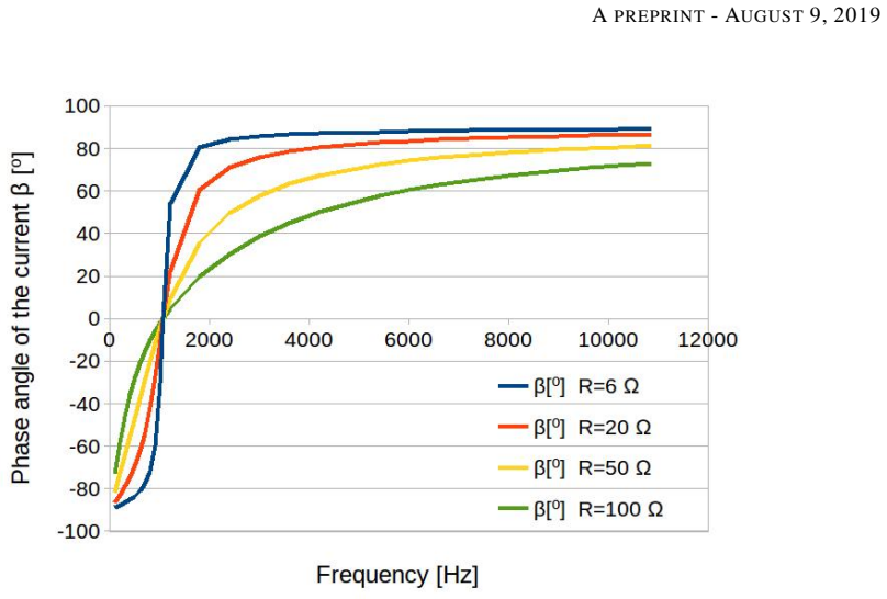
[Section 4, Tables 2 and 3] The text states that phase angles were computed for R = 10, 20, 50, and 100 Ω, but Table 2 is labeled with R = 6 Ω and R = 20 Ω, and Table 1 also uses R = 6 Ω. The resistance values used in the experiment and in the tables should be made consistent.
[Section 2, Equations (2)-(4)] Equation (3) defines i(t) = dq/dt, and the following text says 'replace the Expression (2) in Equation (3)', which is grammatically confusing because Eq. (2) already contains i(t). Rewriting the substitution step would improve clarity.
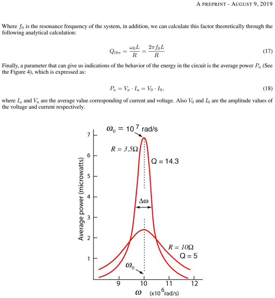
[Figure 4] The caption and the parameters C = 2.0 nF and L = 5.0 µH do not match the experimental component values used elsewhere in the paper. If Figure 4 is an illustrative calculation, the caption should state this explicitly.
[Introduction and References] Several cited references, such as the memristive amoeba-learning paper, appear unrelated to the RLC laboratory experiment and to the educational claims. Adding a few standard RLC-circuit laboratory references would improve the pedagogical grounding.

Circularity Check

3 steps flagged · score 6.0 of 10

Claimed inverse parameter extraction is never performed; theoretical resonance, phase angles, and Q are computed from the same nominal L, C, R values that the inverse model was supposed to recover.

fitted input called prediction [Section 3, Experimental study, Step 1]
"1. For the values of L = 4, 83 mH and C = 4, 7 µF given, calculate the theoretical value of the resonant frequency of the circuit, according to the Equation (9)."

The paper's central claim is that R, L, and C can be obtained from current and voltage measurements through an inverse model. Here, however, the supposedly unknown L and C are given inputs used to compute the resonance frequency. Any subsequent ‘predicted’ resonance or Q value is therefore a forward calculation from the assumed parameters, not an inverse estimate from the data.
self definitional [Section 4, first paragraph; Eq. (15); Tables 2 and 3]
"Once we take the experimental data of the current in the series RLC circuit, using equation (15), we can obtain the value of the phase angle for the charge α =−β and the angular shift of the current β."

Equation (15), tan(β) = (Lω − 1/(cω))/R, is a forward formula that already requires R, L, and C. The phase angles in Tables 2 and 3 are computed from this formula using the same nominal L and C values and the four chosen R values. Thus the phase-angle ‘results’ are not extracted from the measured current data; they are the theoretical model evaluated at the very parameters the inverse method was supposed to discover.

1 more flagged steps

fitted input called prediction [Section 4, Table 4 and surrounding text]
"Also, we show in table 4 the results of the experimental and theorical quality factor Q (See the equations (16) and (17)) for the four resistances, based on the frequency values f1 and f2 using Figure 5."

The theoretical quality factor is Q_the = ω0L/R, computed from the nominal L and R values and the nominal resonance frequency. The experimental quality factor Q_exp = f0/(f2−f1) is read from the measured resonance curve. Comparing these two quantities validates a forward model with assumed parameters; it does not demonstrate inverse recovery of R, L, or C from the measurements. The large 25.4% error at R = 100 Ω further shows that even this forward-model check is weak in one regime.

full rationale

The underlying circuit theory (Kirchhoff's law, the damped driven oscillator analogy, impedance, phase, and quality factor) is standard and self-contained, with no self-citation or imported uniqueness theorem. The circularity lies in the advertised inverse-model demonstration: Section 3 Step 1 uses the given L and C to precompute the resonance frequency; Section 4 computes all phase angles from Eq. (15) using those same nominal parameters; and Table 4 computes Q_the from nominal L and R while Q_exp is read from the same measured current curve. The claimed extraction of R, L, and C from current and voltage measurements is never actually performed, and no voltage measurements or Python analysis are reported. What is presented is therefore a forward-model consistency check between the measured resonance curve and values generated from the assumed circuit parameters, so the central claim of inverse parameter recovery reduces by construction to using those parameters as inputs.

Assumptions & free parameters 0 free parameters · 3 assumptions · 0 invented entities

The central claim requires no fitted constants because the inverse extraction is never carried out. The only assumptions are ideal circuit behavior and the standard resonance formulas, plus the unstated accuracy of the manual current measurements.

assumptions (3)

domain assumption Kirchhoff's mesh law applies to the series RLC circuit with ideal lumped components.
Equation (1) writes V(t) = VR + VL + VC as a sum over ideal resistor, inductor, and capacitor; parasitic resistances and source impedance are ignored.
standard math The steady-state sinusoidal solution of the forced damped oscillator equation applies, giving impedance division and phase relations in Eqs. (10), (14), and (15).
The paper compares Eq. (7) to Eq. (8) and uses the complex impedance result without derivation.
domain assumption The experimentally measured current values are accurate enough that f1 and f2 from the resonance curve define Q_exp via Eq. (16).
No error bars are given for the current measurements, and the bandwidth points are read from plotted curves.

how reviews work

0 comments

Cite this review

Pith. "Pith review of Teaching Forced Damped Oscillator Using RLC Circuit Through Inverse Modeling." pith.science (2026). https://pith.science/paper/BB53YUXE

@misc{pith2026190801891,
  author       = {Pith},
  title        = {Pith review of: Teaching Forced Damped Oscillator Using RLC Circuit Through Inverse Modeling},
  year         = {2026},
  howpublished = {\url{https://pith.science/paper/BB53YUXE}},
  note         = {Machine review of arXiv:1908.01891}
}

read the original abstract

Teaching by direct models in science has been weakening the learning process of the students, because the real problems in engineering are not solved by direct models instead commonly they are solved by inverse models. On the other hand, one of the most relevant topics in the course of waves and particle physics oriented for the forming engineers; it's the subject of simple harmonic motion forced damping, which many physical phenomena can be explained as the quality factor Q and the resonance frequency of an oscillatory forced system. In order to capture the attention of students and give an application to this issue. We have developed an experimental setup to take measurements of electric current, voltages from capacitor and inductor for different frequencies and resistances, once the experimental data were collected to study the behavior of the electrical current inside the circuit and find out the RLC parameters with an inverse model. Finally, we want to show the process in detail how parameters of the system (Resistance, Inductance and Capacitance values) are very relevant in this kind of systems, from the results obtained by experimental measurements of voltage, current and angle of phase shift, where this was achieved by implementing an indirect method described in this document, so that can be applied to studies of more complex systems such as a motor where such parameters may be unknown.

Figures

Figures reproduced from arXiv: 1908.01891 by the authors.

**Figure 2.** Graph of the current as a function of the frequency, where the expected behavior for three resistances of [PITH_FULL_IMAGE:figures/full_fig_p003_2.png] view at source ↗

**Figure 3.** Beta angle behavior β for two different resistance values in a series RLC circuit, where the black curve belongs to the value of the lowest value resistance R1, so the curve of red color corresponds to the resistance of greater value R2 (R2 > R1). One of the most important parameters to be calculated in this type of systems (serial RLC circuit), is the quality factor or merit factor denoted also as factor Q, is defi… view at source ↗

Figures from the paper (4 more)

**Figure 4.** Figure 4: Calculation of the average power of an RLC circuit for the following parameters: [PITH_FULL_IMAGE:figures/full_fig_p005_4.png]

**Figure 5.** Figure 5: Graph of the current as a function of the frequency of the RLC circuit in series for four different resistance [PITH_FULL_IMAGE:figures/full_fig_p007_5.png]

**Figure 6.** Figure 6: Phase angle of the electric charge, stored in the RLC circuit in series as a function of the frequency for four [PITH_FULL_IMAGE:figures/full_fig_p008_6.png]

**Figure 7.** Figure 7: Phase angle of the electric current, circulating in the RLC circuit in series as a function of the frequency for [PITH_FULL_IMAGE:figures/full_fig_p009_7.png]

Discussion (0). Continue with ORCID to comment.

Reference graph

Works this paper leans on

11 extracted references · 11 canonical work pages

[1]

V., La Fontaine, S., & Di Ventra, M

Pershin, Y. V., La Fontaine, S., & Di Ventra, M. (2009). Memristive model of amoeba learning. Physical Review E, 80(2), 021926

work page 2009
[2]

Comi, C., Corigliano, A., Langfelder, G., Longoni, A., Tocchio, A., & Simoni, B. (2010). A resonant microaccelerometer with high sensitivity operating in an oscillating circuit. Journal of microelectromechanical systems, 19(5), 1140-1152

work page 2010
[3]

Flanagan, J., & Landgraf, L. (1968). Self-oscillating source for vocal-tract synthesizers. IEEE Transactions on Audio and Electroacoustics, 16(1), 57-64

work page 1968
[4]

Ibrahim, D. (2011). Engineering simulation with MATLAB: improving teaching and learning effectiveness. Procedia Computer Science, 3, 853-858

work page 2011
[5]

Herniter, M., Scott, D., & Pangasa, R. (2001). Teaching programming skills with MATLAB. age, 6, 1

work page 2001
[6]

A., & Concari, S

Kofman, H. A., & Concari, S. B. (2012). Using remote lab for physics teaching. J. García Zubía, & G. Alves (comp.), Using remote labs in education, 293-308

work page 2012
[7]

Sears, Z. (1976). Young, University Physics

work page 1976
[8]

A., Jewett, J

Serway, R. A., Jewett, J. W., Hernández, A. E. G., & López, E. F. (2005). Física para ciencias e ingeniería (Vol. 6). Thomson

work page 2005

Show all 11 references

[9]

S., & Cullen, M

Zill, D., Wright, W. S., & Cullen, M. R. (2011). Advanced engineering mathematics. Jones & Bartlett Learning

2011
[10]

A., & Mosca, G

Tipler, P. A., & Mosca, G. (2007). Physics for scientists and engineers. Macmillan

2007
[11]

Janert, P. K. (2010). Gnuplot in action: understanding data with graphs. Manning

2010

Pith tools

Reviewed August 14, 2026 · model on record in the stance chip above.

[1] [1]

V., La Fontaine, S., & Di Ventra, M

Pershin, Y. V., La Fontaine, S., & Di Ventra, M. (2009). Memristive model of amoeba learning. Physical Review E, 80(2), 021926

work page 2009

[2] [2]

Comi, C., Corigliano, A., Langfelder, G., Longoni, A., Tocchio, A., & Simoni, B. (2010). A resonant microaccelerometer with high sensitivity operating in an oscillating circuit. Journal of microelectromechanical systems, 19(5), 1140-1152

work page 2010

[3] [3]

Flanagan, J., & Landgraf, L. (1968). Self-oscillating source for vocal-tract synthesizers. IEEE Transactions on Audio and Electroacoustics, 16(1), 57-64

work page 1968

[4] [4]

Ibrahim, D. (2011). Engineering simulation with MATLAB: improving teaching and learning effectiveness. Procedia Computer Science, 3, 853-858

work page 2011

[5] [5]

Herniter, M., Scott, D., & Pangasa, R. (2001). Teaching programming skills with MATLAB. age, 6, 1

work page 2001

[6] [6]

A., & Concari, S

Kofman, H. A., & Concari, S. B. (2012). Using remote lab for physics teaching. J. García Zubía, & G. Alves (comp.), Using remote labs in education, 293-308

work page 2012

[7] [7]

Sears, Z. (1976). Young, University Physics

work page 1976

[8] [8]

A., Jewett, J

Serway, R. A., Jewett, J. W., Hernández, A. E. G., & López, E. F. (2005). Física para ciencias e ingeniería (Vol. 6). Thomson

work page 2005