REVIEW 3 major objections 4 minor 34 references
A new unified stabilized mixed finite element method of the Stokes-Darcy coupled problem: Isotropic discretization
T0 review · 3 major / 4 minor · reviewed 2026-08-14 · deepseek-v4-flash
Pith's one-line read A single nonconforming Crouzeix-Raviart element, with normal-only continuity in the Darcy region, yields an optimally convergent stabilized mixed method for coupled Stokes-Darcy flow.
desk verdict Nice idea—cheaper unified Stokes–Darcy element—but the interpolation lemma for the enlarged space is unproved and the Fortin argument doesn't go through, so the convergence theorem is unsupported. read the letter →
The pith
A machine-rendered reading of the paper's core claim, the machinery that carries it, and where it could break.
The reading
What carries the argument
The two devices that carry the argument are the modified Darcy formulation and the enlarged Crouzeix-Raviart space $H_h$. The Darcy modification replaces the raw momentum equation by $(\mu K^{-1}u,v)_{\Omega_d} + (\mathrm{div}\,u,\mathrm{div}\,v)_{\Omega_d}$ plus pressure terms, which makes the bilinear form coercive over the relevant $H(\mathrm{div})$ space and allows the same element in both regions. The space $H_h$ defined in (28)-(29) requires average continuity of the entire velocity across edges in the Stokes region and of only the normal component across edges in the Darcy region and on the outer Darcy boundary; a stabilization term $J(u,v)$ with $h^{-1}$ weights penalizes the remaining jumps. The convergence proof combines the discrete inf-sup condition with interpolation estimates for the four face-integral consistency errors.
What would settle it
Compute the interpolation operator $r_h$ defined by (49)-(50) on a single isotropically refined mesh in two dimensions, using a Darcy-region velocity that has a nonzero tangential average jump across an interior edge; if $\|r_h v\|_h$ grows faster than a constant times $\|v\|_{1,d}$ as the mesh is refined, Lemma 3.2 is false and Theorem 3.4 is unsupported. Alternatively, run the Section 4 numerical test with a Darcy velocity in $H(\mathrm{div})$ but not $H^1$ to see whether the claimed $O(h)$ rate collapses.
Extended reading notes
Core claim
The central claim is Theorem 3.4: if the exact velocity is $H^2$ in each subdomain and the pressures are $H^1$, then the finite element solution satisfies $\|u-u_h\|_h + \|p-p_h\| \leq C h (|u|_{2,s}+|u|_{2,d}+|p|_{1,s}+|p|_{1,d})$, with $C$ independent of the mesh size. The method achieves this by modifying the Darcy problem with an added $\mathrm{div}$-$\mathrm{div}$ term and by using a Crouzeix-Raviart space that enforces zero mean jump of the full velocity on Stokes-side edges but only zero mean jump of the normal component on Darcy-side edges, which is the natural continuity for $H(\mathrm{div})$ velocity fields. The discrete inf-sup condition is proved via a Fortin argument, and the error analysis handles the resulting nonconformity through explicit face-integral estimates.
Load-bearing premise
The convergence proof assumes that the interpolation operator onto the enlarged space $H_h$ is bounded in the discrete norm and that the quoted approximation estimates hold, but these properties were proven for a smaller space in a cited paper and are not verified for the normal-continuity-only Darcy space actually used.
Editorial extensions
If this is right
- The discrete problem (31) is well-posed for any regular, interface-conforming triangulation, yielding a unique velocity-pressure pair in $H_h\times Q_h$.
- For smooth solutions the method reaches the optimal first-order convergence rate in the discrete norm, so halving the mesh size halves the combined velocity-pressure error.
- Because the same nonconforming element is used in both regions and the pressure is piecewise constant, the implementation is simpler than methods that pair different stable elements in the Stokes and Darcy domains.
- The stabilization term that penalizes element-edge jumps is essential to the coercivity proof, so the scheme avoids the need for separate inf-sup stable pairs in each subdomain.
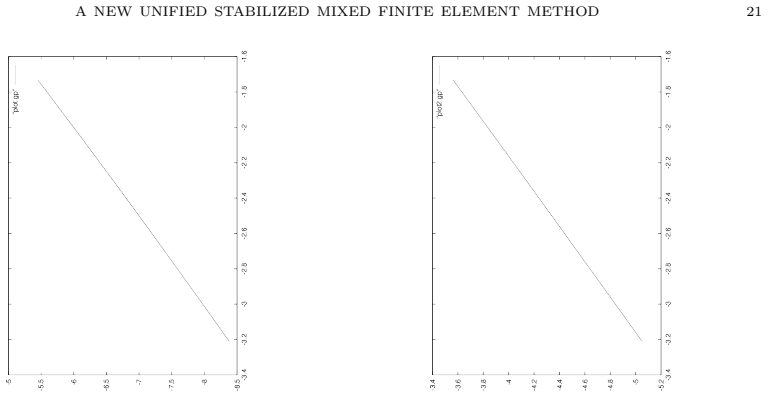
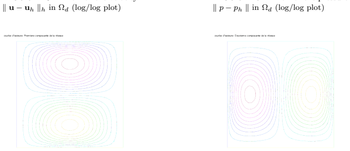
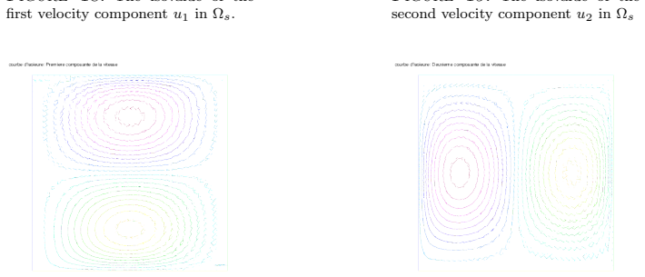
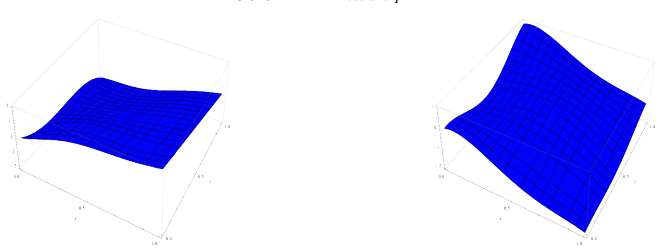
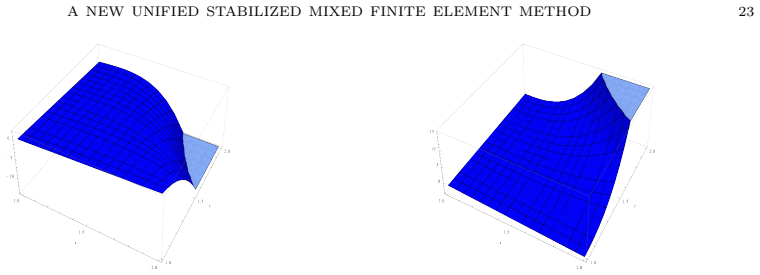
- The numerical experiment on a two-dimensional model problem reproduces the predicted first-order convergence rates for both velocity and pressure.
Reading between the lines
- If the missing interpolation bound for $H_h$ can be established directly rather than quoted from a smaller space, the same scheme would be fully self-contained and likely extend to anisotropic meshes, since jump-penalty terms similar to discontinuous Galerkin methods often tolerate anisotropy.
- The added $\mathrm{div}$-$\mathrm{div}$ term in the Darcy modification is a natural stabilization that vanishes on exactly divergence-free Darcy velocities; this suggests the method may transfer to a Brinkman-type model where the same term acts as a consistent penalty.
- A test with Darcy velocity in $H(\mathrm{div})$ but not $H^1$ would reveal whether the $O(h)$ rate depends on the stronger smoothness assumption or whether the normal-only continuity already captures the true regularity of the solution.
- The face-integral estimates in Lemma 3.5 are written for isotropic meshes; porting them to anisotropic meshes would require a trace inequality with explicit dependence on element aspect ratios, which could be the next step toward a unified anisotropic analysis.
Signed reviews
Editorial analysis
A structured set of objections, weighed in public.
Referee Report
Summary. The manuscript proposes a unified stabilized mixed finite element method for the coupled Stokes–Darcy problem. The Darcy equation is modified by adding a div-div term, and both subproblems are discretized with a variant of the nonconforming Crouzeix–Raviart element in a single velocity space, with full-vector jump vanishing only in the Stokes region and normal-component jump vanishing in the Darcy region and on its boundary, together with a jump stabilization term. The paper claims well-posedness of the discrete problem, a discrete inf-sup condition, and an optimal first-order a priori error estimate under H^2/H^1 regularity, and reports one numerical experiment in two dimensions that shows the expected convergence behavior.
Significance. If the proof were completed, the result would be genuinely useful: it would justify a cheap, unified nonconforming discretization in which the Darcy velocity space only approximates H(div), which is more natural than enforcing full H^1 continuity in the porous medium. The scheme itself and the stabilization are reasonable, and the numerical experiment is consistent with the claimed rate. However, the central convergence argument depends on an interpolation operator that is not shown to map into the actual discrete space and is deferred to a reference that treats a smaller space. As written, the discrete inf-sup condition and the convergence theorem are not established. The contribution is promising, but the missing proof is load-bearing and requires a substantive repair.
major comments (3)
- [Section 3.1, Lemma 3.2 and equations (28)-(29), (49)-(50)] The interpolation operator r_h defined by (49)-(50) is not shown to map W into the actual space H_h. H_h in (28)-(29) requires full-vector jump moments to vanish on E_h(Ω_s^+) and normal-component jump moments to vanish on E_h(Ω_d) ∪ E_h(∂Ω_d), whereas (49)-(50) only fix edge moments on E_h(Ω_s) and E_h(Ω_d). In particular, the boundary-edge conditions on Γ_s, Γ_d, and Γ_I are not imposed by (49)-(50): for v∈W with v=0 on Γ_s and v·n_d=0 on Γ_d, there is no reason that r_h v satisfies the corresponding discrete conditions. Since Lemma 3.2 is proved only by saying "similar to [30]" and the space in [30] is smaller, the boundedness of r_h in the discrete norm is unproved for the enlarged H_h. This lemma underpins both the Fortin argument and the approximation estimate in Lemma 3.4, so the O(h) claim in Theorem 3.4 is unsupported as written.
- [Section 3.1, Theorem 3.2 (Fortin argument)] The Fortin proof integrates by parts over all elements and then restricts the resulting jump sum to E_h(Ω_s^+) ∪ E_h(Ω_d), omitting the edges in E_h(∂Ω_d). Because r_h v is not known to lie in H_h, the boundary terms on Γ_d and Γ_I are not zero, so the identity b_h(r_h v, q_h) = b_h(v, q_h) does not follow from (49)-(50). For v∈[H^1_0(Ω)]^N, the term Σ_{E⊂∂Ω_d} ∫_E q_h n_E·(r_h v) is generally nonzero unless additional conditions are imposed on r_h. Thus the discrete inf-sup condition (52) is not established.
- [Section 3.1, Theorem 3.1 and equations (43)-(47)] The coercivity proof contains some nontrivial steps that are only sketched: the transition from (42) to (43) and then to (44) relies on a discrete Korn inequality for a space with mixed jump conditions, but the precise hypotheses under which [5] applies to H_h are not stated. In addition, the inequalities in (45)-(47) use the symbol ">" where a lower bound with a constant is intended. These issues are repairable, but they add to the impression that the well-posedness proof is not fully self-contained.
minor comments (4)
- [Section 3.2, Lemma 3.5] The expressions ([v_h·n_E, p_s]_E)_E and ([v_h·n_E, p_d]_E)_E are typographically confusing; they should be written as ([v_h·n_E]_E, p_s)_E and ([v_h·n_E]_E, p_d)_E, respectively.
- [Section 3.2, Theorem 3.4] The final bound in (72) contains the typo |u2,d; it should read |u|_{2,d}. The word "satisfies" is also misspelled in the theorem statement.
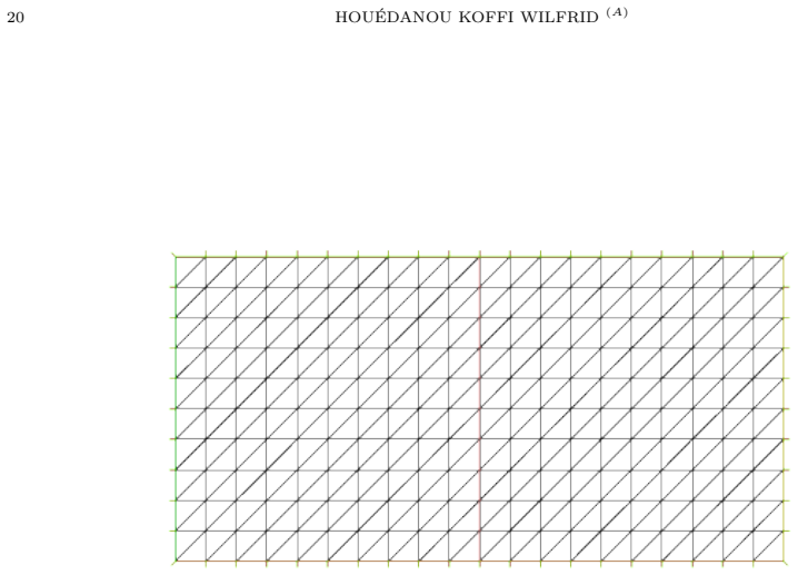
- [Section 4, numerical experiments] Only one numerical test is reported, and the observed convergence orders are not extracted or tabulated. Reporting the empirical orders for ‖u−u_h‖_h and ‖p−p_h‖ would make the numerical confirmation of the O(h) claim more convincing.
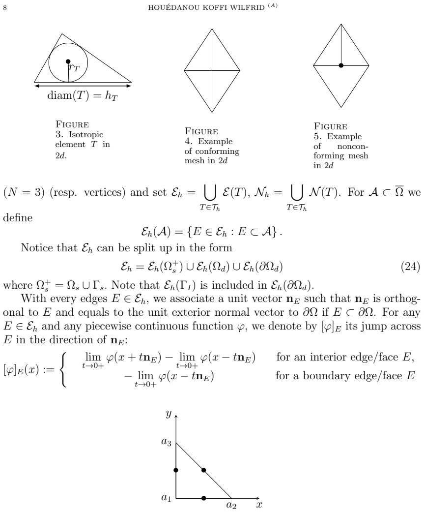
- [Section 3.1, notation] The decomposition E_h = E_h(Ω_s^+) ∪ E_h(Ω_d) ∪ E_h(∂Ω_d) in (24) should be stated with a short explanation that E_h(Ω_s^+) includes Γ_s, while E_h(∂Ω_d) includes Γ_d and Γ_I; this would help the reader see exactly which jump terms are penalized.
Circularity Check
No circular reduction: the discrete error analysis is derived in-paper; deferred interpolation lemmas create a correctness gap, not circularity.
full rationale
The central claim, Theorem 3.4, is an a priori error bound obtained through a standard Strang-lemma chain. Coercivity (Theorem 3.1), the Fortin-based discrete inf-sup condition (Theorem 3.2), and the consistency term estimates (Lemma 3.5) are argued in the paper; no fitted parameter is renamed as a prediction, and no equation defines the predicted convergence rate as an input. Theorem 2.1 is attributed to the author's earlier work [27], but it is a standard mixed well-posedness result whose proof ingredients (continuity, inf-sup, coercivity plus classical mixed theory) are indicated in the text, and it does not by construction imply the discrete O(h) bound. The numerical experiment manufactures an exact solution and solves for the corresponding right-hand sides, so the observed rates are independent checks rather than fits. The main weakness flagged in the derivation—Lemma 3.2 and Lemma 3.4 are deferred to [30] while the present H_h is larger, requiring only normal continuity on Darcy edges—is a verification and correctness gap, not a circular reduction: nothing in the paper equates the target error with the assumed interpolation bound by definition. Accordingly, per the hard rules, this is not circularity.
Assumptions & free parameters
free parameters (1)
- Stabilization coefficient =
(1+2\mu) in J_{\Omega_s^+}; 1 in J_{\Omega_d} and J_{\partial\Omega_d}
assumptions (6)
- standard math Continuous well-posedness of the modified variational problem (21) (Theorem 2.2).
- standard math Boundedness of the Crouzeix-Raviart interpolant r_h in the discrete norm (Lemma 3.2).
- standard math Discrete Korn inequality for piecewise H^1 functions, applied in Theorem 3.1.
- domain assumption Shape-regular conforming triangulations aligned with the Stokes/Darcy subdomains.
- domain assumption The permeability tensor K is symmetric, uniformly positive definite with bounds K_* and K^*; the source g has zero mean.
- standard math Existence of a Fortin operator for the pair (H_h, Q_h) and standard interpolation error estimates.
Cite this review
Pith. "Pith review of A new unified stabilized mixed finite element method of the Stokes-Darcy coupled problem: Isotropic discretization." pith.science (2026). https://pith.science/paper/7UBUUBXD
@misc{pith2026190801892,
  author       = {Pith},
  title        = {Pith review of: A new unified stabilized mixed finite element method of the Stokes-Darcy coupled problem: Isotropic discretization},
  year         = {2026},
  howpublished = {\url{https://pith.science/paper/7UBUUBXD}},
  note         = {Machine review of arXiv:1908.01892}
}
abstract
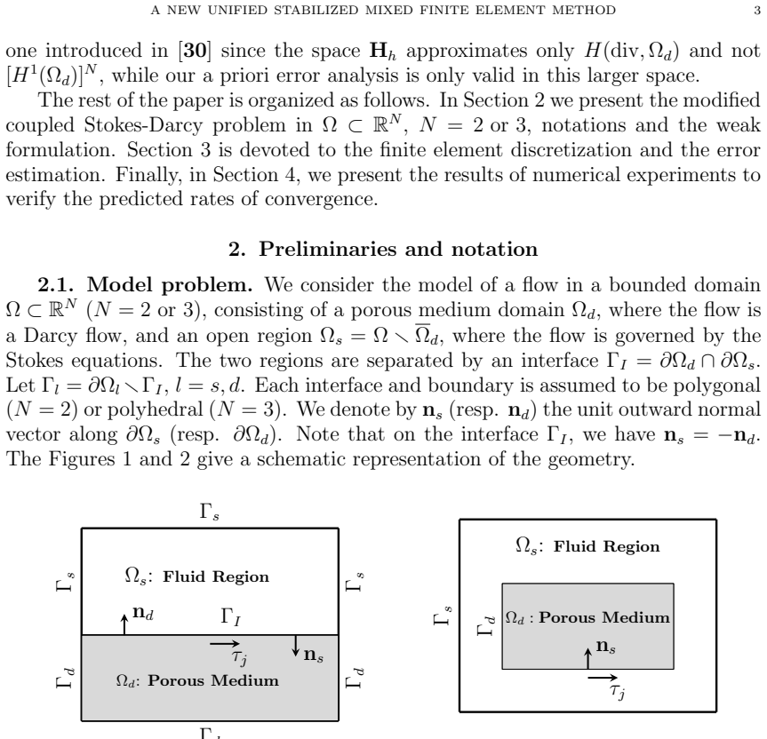
In this paper we develop an a priori error analysis of a new unified mixed finite element method for the coupling of fluid flow with porous media flow in $\mathbb{R}^N$, $N\in\{2,3\}$ on isotropic meshes. Flows are governed by the Stokes and Darcy equations, respectively, and the corresponding transmission conditions are given by mass conservation, balance of normal forces, and the Beavers-Joseph-Saffman law. The approach utilizes a modification of the Darcy problem which allows us to apply a variant nonconforming Crouzeix-Raviart finite element to the whole coupled Stokes-Darcy problem. The well-posedness of the finite element scheme and its convergence analysis are derived. Finally, the numerical experiments are presented, which confirm the excellent stability and accuracy of our method.
Figures

Figures from the paper (10 more)


Reference graph
Works this paper leans on
- [30]
-
[5]
S. Brenner. Korn’s inequalities for piecewise H 1 vector fields. Math. Comput., 73:1067–1087, 2003
work page 2003
-
[1]
T. Arbogast and D. Brunson. A computational method for approximating a Darcy-Stokes system governing a vuggy porous medium. Computational Geosciences, 11:207–218, 2007
work page 2007
-
[2]
M. G. Armentano and M. L. Stockdale. A unified mixed finite element approximations of the Stokes-Darcy cou- pled problem. Computers and Mathematics with Applications , https://doi.org/10.1016/j.camwa.2018.12.032, 2018
-
[3]
Babuˇ ska and G
I. Babuˇ ska and G. Gatica. A residual-based a posteriori error estimator for the Stokes-Darcy coupled problem. SIAM J. Numer. Anal. , 48:498–523, 2010
2010
-
[4]
G. Beavers and D. Joseph. Boundary conditions at a naturally permeable wall. J. Fluid Mech. , 30:197–207, 1967
work page 1967
-
[6]
W. Chen and Y. Wang. A posteriori error estimate for H(div) conforming mixed finite element for the coupled Darcy-Stokes system. Journal of Computational and Applied Mathematics , 255:502–516, 2014
work page 2014
-
[7]
M. Crouzeix and P. Raviart. Conforming and nonconforming finite element methods for solving the stationary Stokes equations. Rev. Fran¸ caise Automat. Informat. Recherche Op´ erationnelle s´ er. Rouge, 7:33–75, 1973
work page 1973
Show all 34 references
-
[8]
Cui and N
M. Cui and N. Yan. A posteriori error estimate for the Stokes-Darcy system. Math. Meth. Appl. Sci. , 34:1050– 1064, 2011
2011
-
[9]
Discacciati and A
M. Discacciati and A. Quarteroni. Navier-Stokes/Darcy coupling: Modeling, analysis, and numerical approxi- mation. Rev. Math. Comput. , 22:315–426, 2009
2009
-
[10]
A. Ern. Aide-m´ emoire el´ ements finis.Dunod, Paris, ISBN 2 10 007303 6 , 2005
2005
-
[11]
Frederic and P
H. Frederic and P. Olivier. Freefem++. http://www.freefem.org
-
[12]
Galvis and M
J. Galvis and M. Sarkis. Nonconforming mortar discretization analysis for the coupling Stokes-Darcy equations. Electronic. Trans. Numer. Anal., 26:350–384, 2007
2007
-
[13]
Gatica, R
G. Gatica, R. Oyarz` ua, and F.-J. Sayas. A residual-based a posteriori error estimator for a fully-mixed formu- lation of the Stokes-Darcy coupled problem. Comput. Methods Appl. Mech. Engrg. , 200:1877–1891, 2011
2011
-
[14]
G. N. Gatica, S. Meddahi, and R. Oyarz` ua. A conforming mixed finite element method for the coupling of fluid flow with porous media flow. IMA J. Numer. Anal. , 29:86–108, 2009
2009
-
[15]
Gatica, R
G.-N. Gatica, R. Oyarz` ua, and F.-J. Sayas. Convergence of a family of galerkin discretizations for the Stokes- Darcy coupled proplem
-
[16]
Girault and P.-A
V. Girault and P.-A. Raviart. Finite element methods for Navier-Stokes equations, Theory and algorithms , volume 5 of Springer, Berlin. In Computational Mathematics, 1986
1986
-
[17]
F. Hecht. The mesh adapting software: bamg. INRIA report.http://www- c.inria.fr/gamma/cdrom/www/bamg/eng.htm, 1998. 24 HOU ´EDANOU KOFFI WILFRID (A)
1998
-
[18]
K. W. Hou´ edanou, J. Adetola, and B. Ahounou. Residual-based a posteriori error estimates for a conform- ing finite element discretization of the Navier-Stokes/Darcy coupled problem. Journal of Pure and Applied Mathematics : Advances and Applications , 18(1):37–73, 2017
2017
-
[19]
K. W. Hou´ edanou and B. Ahounou. A posteriori error estimation for the Stokes-Darcy coupled problem on anisotropic discretization. Math. Meth. Appl. Sci. , 2016. http://dx.doi.org/10.1002/mma.4261 (in press)
2016 doi
-
[20]
J¨ ager and A
W. J¨ ager and A. Mikeli´ c. On the boundary conditions of the contact interface between a porous medium and a free fluid. Ann. Scuola Norm. Sup. Oisa Cl. Sci. , 23:403–465, 1996
1996
-
[21]
J¨ ager and A
W. J¨ ager and A. Mikeli´ c. On the interface boundary condition of Beavers, Joseph and Saffman.SIAM Journal on Applied Mathematics , 60:1111–1127, 2000
2000
-
[22]
J¨ ager and A
W. J¨ ager and A. Mikeli´ c. On the interface boundary condition of Beavers, Joseph and Saffman.SIAM J. Appl. Math., 60:1111–1127, 2000
2000
-
[23]
J¨ ager, A
W. J¨ ager, A. Mikeli´ c, and N. Neuss. Asymptotic analysis of the laminar visous flow over a porous bed.SIAM J. Sci. Comput. , 22:2006–2028, 2001
2006
-
[24]
R. Li, J. Li, Z. Chen, and Y. Gao. A stabilized finite element method based on two local gauss integrations for a coupled Stokes-Darcy problem. http://dx.doi.org/10.1016/j.cam.2015.06.014, 2015
2015 doi
-
[25]
Mardal, X
K.-A. Mardal, X. Tai, and R. Winther. A robust finite element method for darcy-stokes flow. SIAM Journal on Numerical Analysis, 40:1605–1631, 2002
2002
-
[26]
Mu and J
M. Mu and J. Xu. A two-grid method of a mixed Stokes-Darcy model for coupling fluid flow with porous media flow. SIAM Journal on Numerical Analysis , 45:1801–1813, 2007
2007
-
[27]
Nicaise, B
S. Nicaise, B. Ahounou, and W. Hou´ edanou. A residual-based posteriori error estimates for a nonconforming finite element discretization of the Stokes-Darcy coupled problem: Isotropic discretization. Afr. Mat., African Mathematical Union and Springer-Verlag Berlin Heidelberg: ...
2016
-
[28]
Payne and B
L. Payne and B. Straughan. Analysis of the boundary condition at the interface between a viscous fluid and a porous medium and related modeling questions. J. Math. Pures Appl. , 77:317–354, 1998
1998
-
[29]
Rivi` ere and I
B. Rivi` ere and I. Yotov. Locally conservative coupling of Stokes and Darcy flows. SIAM J. Numer. Anal. , 42:1959–1977, 2005
1959
-
[31]
P. Saffman. On the boundary condition at the interface of a porous medium. Stud. Appl. Math., 1:93–101, 1971
1971
-
[32]
Vassilev and I
D. Vassilev and I. Yotov. Coupling Stokes-Darcy flow with transport. SIAM J. Sci. Comput. , 5:3661–3684, 2009
2009
-
[33]
L. J. William, S. Friedhelm, and Y. Ivan. Coupling fluid flow with porous media flow. SIAM J. Numer. Anal. , 40(6):2195–2218 (2003), 2002
2003
-
[34]
J. Yu, M. A. A. Mahbub, F. Shi, and H. Zheng. Stabilized finite element method for the stationary mixed Stokes- Darcy problem. Advances in Diffference Equations, https:// doi.org/10.1186/s13662-018-1809-2346, 2018. E-mail address: a) khouedanou@yahoo.fr D´epartement de Math´emat...
2018 doi
Reviewed August 14, 2026 · model on record in the stance chip above.
Discussion (0). Continue with ORCID to comment.