REVIEW 3 major objections 4 minor 18 references
Fast Time-optimal Avoidance of Moving Obstacles for High-Speed MAV Flight
T0 review · 3 major / 4 minor · reviewed 2026-08-14 · deepseek-v4-flash
Pith's one-line read This paper claims a planner that lets a fast-flying micro aerial vehicle dodge a suddenly perceived moving obstacle by inserting a viastate at an obstacle corner, while keeping the trajectory time-optimal and dynamically feasible.
desk verdict A genuinely fast viastate-based avoidance pipeline with a real but qualified optimality claim; the paper itself concedes the 'time-optimal' label only holds under zero-acceleration corner viastates. read the letter →
The pith
A machine-rendered reading of the paper's core claim, the machinery that carries it, and where it could break.
The reading
What carries the argument
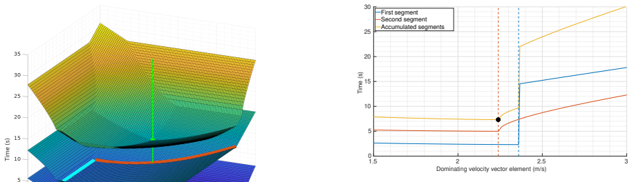
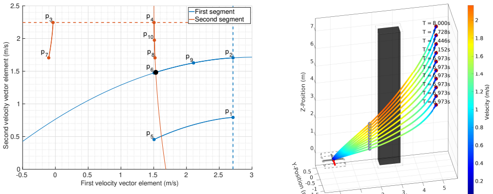
The central object is the viastate: a full state (position, velocity, acceleration) inserted between start and target, turning one trajectory into two segments that meet at an obstacle corner. The paper's key identity is the cost-surface structure of the two segments: for each bound axis, the time of a segment as a function of the viastate velocity has a single minimum and a plateau, so the total-time optimum is either the minimum of the dominant axis or the intersection of two quadratic polynomials fit through sampled points near the optimum. This, together with a database of closed-form solutions for the trajectory-shape equations (the 21 second-order conditions for the seven constant-jerk phases), is what lets the planner evaluate candidate trajectories in microseconds rather than milliseconds per sample.
What would settle it
Run a brute-force grid search over viastate velocities (as the paper itself does to visualize the cost surface) in a scenario where the obstacle is large and close to start or target, and compare the best grid trajectory with the planner's chosen trajectory; if any grid velocity yields a lower total time than the proposed root of the quadratic polynomials, the claim of time-optimality is disproved for that case.
Extended reading notes
Core claim
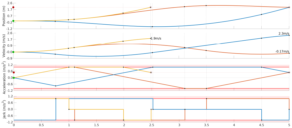
On the paper's own terms, the discovery is an algebraic shortcut for the otherwise expensive problem of choosing an optimal intermediate state. The authors model the MAV as a triple integrator with per-axis limits on velocity, acceleration, and jerk, and generate bang-singular-bang trajectories as concatenations of up to seven constant-jerk phases, with all closed-form solutions stored in a database. When the nominal trajectory collides with an axis-aligned cuboid, two 'bound' axes are chosen and the viastate position is fixed at the obstacle corner pushed out by the vehicle radius plus margin; the viastate acceleration is set to zero. The remaining degree of freedom is the two-element velocity vector at the viastate. The paper argues that the total time splits into two segments whose cost surfaces have characteristic 'grooves', and that the globally optimal velocity lies either at the extremum of a single dominant component or at the intersection of two quadratic polynomials fitted through three sample points per segment. This reduces what would require tens of thousands of trajectory evaluations to a handful of closed-form solves, with the whole avoidance pipeline, including collision checking, finishing in 5.98 ms in the reported scenario.
Load-bearing premise
The claimed time-optimality rests on the assumption that the fastest evasive path belongs to the family of trajectories that pass through a corner of the obstacle with zero acceleration; if the true optimum accelerates through the corner, the generated trajectories are not time-optimal.
Editorial extensions
If this is right
- A drone that perceives an obstacle suddenly can begin an avoidance maneuver within milliseconds, so the method can run as a low-level layer at typical control-loop frequencies.
- Obstacles can be static or moving, and because the method treats each axis independently, the same pipeline works in four or more dimensions, e.g., adding yaw to handle constraints like 'do not look in direction X while inside volume Y'.
- The number of candidate evasions grows as $p = n!/(n-2)!$ in $n$ dimensions, and each candidate is independent, so the computation parallelizes across cores.
- Even though trajectories are time-optimal, the method can be used in a replanning loop: if the fastest candidate collides with another obstacle, the next fastest is selected, and uncertainty can be absorbed by increasing the obstacle margin and replanning frequently.
Reading between the lines
- The paper leaves implicit that the zero-acceleration viastate is a safety-motivated restriction: it makes the vehicle's state at the closest approach easy to correct, but a small amount of acceleration toward the obstacle could shave off time; an extension would relax this constraint and compare the resulting speedup against the loss of robustness.
- The quadratic-polynomial tradeoff is an approximation fitted through three sampled points; a natural test is to increase the number of samples or use the exact cost-surface curvature to see whether the intersection root is ever more than a few percent suboptimal.
- The axis-aligned cuboid representation can be chained to represent more complex environments as unions of boxes, but the method as presented does not reason about overlapping or non-convex obstacles; extending the selection of bound axes to such unions is a direct next step.
- Because the planner is so fast, it could be used as an inner loop inside a sampling-based or global planner, giving the global planner a fast dynamic-feasibility oracle rather than relying on a separate low-level controller.
Signed reviews
Editorial analysis
A structured set of objections, weighed in public.
Referee Report
Summary. The manuscript proposes a reactive obstacle-avoidance method for micro aerial vehicles (MAVs) built on the authors' earlier trajectory generator for third-order systems. The method first generates a time-optimal trajectory from a full start state to a possibly partially defined target state, checks it for collisions by exploiting the piecewise polynomial form, and, if a collision is found, inserts viastates at obstacle corners. For the two 'bound' axes, the viastate is placed at a projected obstacle corner with zero acceleration, and the viastate velocity is chosen by one of two heuristics: a single dominating velocity component, or a tradeoff computed from the intersection of quadratic polynomials fitted through three sample points. The remaining 'free' axes are synchronized to the bound axes. The paper reports sub-6 ms computation on a single CPU core, a fuzz test of partially defined target states, and over 100 obstacle-avoidance scenarios with one moving-obstacle example.
Significance. If the optimality claim held, the method would be a useful building block for high-speed MAV navigation: it is fast, handles moving axis-aligned cuboids, and produces smooth dynamically feasible trajectories with arbitrary dimensionality. The paper has concrete strengths: the collision check via zero crossings of polynomials is elegant, the solution database for partially defined target states is a practical contribution, the code is announced as open source, and the runtime claim is falsifiable and clearly stated. However, the headline contribution is currently the time-optimality guarantee, and that guarantee is not established: the search space is restricted to corner viastates with zero acceleration, and the multi-velocity tradeoff is solved by a polynomial fit rather than an exact optimization. The significance is therefore conditional on either restricting the claims to the considered family or providing a quantitative bound on the suboptimality gap.
major comments (3)
- [Sec. IV-B.1, Abstract, Conclusion] The unqualified 'time-optimal' claim is not established. The search space for the viastate is restricted to obstacle corners with zero acceleration, and the paper itself states that 'a nonzero acceleration could be slightly faster' and that optimality holds only 'under the assumption of zero acceleration.' No argument or proof is given that the globally fastest trajectory in the considered problem class must pass through a corner, nor that zero acceleration is optimal; this is particularly non-obvious for moving cuboids with asymmetric start and target states. Since the Abstract and Conclusion repeat the unconditioned claim, the central contribution is currently over-stated. The authors should either restrict all optimality claims to the restricted family, or prove that the global optimum lies in that family and quantify any gap.
- [Sec. IV-B.3, Eqs. (8)-(10)] Even within the restricted corner/zero-acceleration family, the optimal viastate velocity is not computed exactly in the multi-velocity case. The method fits second-order polynomials through three sample points and solves for their intersection; the fitted polynomials are an approximation of the true cost landscape, and no error bound or validation against the sampled map (Fig. 4) is provided. The claim that the method 'maintains time-optimality' therefore depends on an unquantified approximation. Please either provide an exact derivation for these cases or evaluate the resulting suboptimality against dense sampling over a range of start/target/obstacle configurations.
- [Sec. V-B] The evaluation as reported is too weak to support the runtime and optimality claims. The 100+ scenarios are not summarized statistically, no performance criteria or pass rates are given, and the only timing experiment is a single profiling run (Fig. 8). There is no comparison to an optimal or reference planner and no optimality-gap measurement, and the fuzz test in Sec. V-A exercises partially defined target states rather than obstacle avoidance. The single moving-obstacle example uses constant motion. Additional randomized experiments with reported distributions, and a comparison against a global optimum or dense sampling, are needed before the headline claims can be accepted.
minor comments (4)
- [Eq. (10)] The variable t in Eq. (10) is not defined in the text; please specify that it is the polynomial variable and describe how the root in the feasible interval is selected.
- [Sec. IV-A and Sec. V-B] Section IV-A says obstacle motion can be described by concatenated polynomials of rank at most three, but Section V-B later says the method 'assumes a constant motion of the obstacle'; please clarify whether accelerating or otherwise non-constant obstacle motion is supported and evaluated.
- [Throughout] The text contains several typographical and formatting issues, including 'an time-optimal' in the Introduction, 'dont't' in the Related Work, and inconsistent spacing in 'MA V'; a careful proofread is needed.
- [Sec. I] The statement that the code is open source points to a video/challenge webpage rather than a direct repository link; please provide the repository URL so the reproducibility claim can be verified.
Circularity Check
No significant circularity: the avoidance pipeline is an application of the authors' prior trajectory generator, and the paper's explicit zero-acceleration corner-viastate assumption is a scope caveat rather than a circular reduction.
full rationale
Walking the derivation chain, the time-optimal trajectories are produced by the authors' previously published generator [5], and Section III extends that generator to partially defined target states by setting up the 21-ODE bang-singular-bang system and solving for the time phases; no quantity is fitted to the paper's own avoidance claims. In Section IV-B.1 the viastate is deliberately restricted to an obstacle corner with zero acceleration, and the paper states: "under the assumption of zero acceleration, the generated evading trajectories are optimal." That sentence is an explicit scope condition, not a circular reduction: the optimizer is solving a well-defined restricted problem, and the abstract's unqualified "maintain time-optimality" is an overstatement of this restricted optimality, which is a correctness/scope issue rather than a logical tautology. The multi-velocity tradeoff in Section IV-B.3 is approximate because it fits second-order polynomials through sampled points and intersects them, but the fitted curves are used as a computational approximation of the optimum, not as a fitted parameter whose output is the claimed prediction. Self-citations to [5], [17], and [18] are heavy, but [5] is used as an openly cited building block for trajectory generation rather than as an imported uniqueness theorem that forbids alternatives, so the central avoidance result does not reduce to its own inputs by construction.
Assumptions & free parameters
free parameters (2)
- Viastate acceleration =
0
- Obstacle padding margin =
not specified
assumptions (5)
- domain assumption MAV dynamics are modeled as a triple integrator with piecewise constant jerk and up to seven phases per trajectory segment.
- domain assumption Obstacles are axis-aligned hyperrectangles whose position, velocity, acceleration over time are polynomials of rank at most 3.
- ad hoc to paper The optimal avoidance trajectory passes through a corner of the obstacle with zero acceleration at the viastate.
- ad hoc to paper The time-optimal viastate velocity for two bound axes can be found by intersecting two quadratic polynomials fitted through three points each.
- domain assumption Collision avoidance can always be achieved by temporally disconnecting two 'bound' axes; free axes are synchronized afterward.
Cite this review
Pith. "Pith review of Fast Time-optimal Avoidance of Moving Obstacles for High-Speed MAV Flight." pith.science (2026). https://pith.science/paper/ZWVQ7SQ3
@misc{pith2026190802028,
  author       = {Pith},
  title        = {Pith review of: Fast Time-optimal Avoidance of Moving Obstacles for High-Speed MAV Flight},
  year         = {2026},
  howpublished = {\url{https://pith.science/paper/ZWVQ7SQ3}},
  note         = {Machine review of arXiv:1908.02028}
}
read the original abstract
In this work, we propose a method to efficiently compute smooth, time-optimal trajectories for micro aerial vehicles (MAVs) evading a moving obstacle. Our approach first computes an n-dimensional trajectory from the start- to an arbitrary target state including position, velocity and acceleration. It respects input- and state-constraints and is thus dynamically feasible. The trajectory is then efficiently checked for collisions, exploiting the piecewise polynomial formulation. If collisions occur, viastates are inserted into the trajectory to circumvent the obstacle and still maintain time-optimality. These viastates are described by position, velocity, and acceleration. The evaluation shows that the computational demands of the proposed method are minimal such that obstacle avoidance can begin within few milliseconds. Optimality of generated trajectories, combined with the ability for frequent online re-planning from non-hover initial conditions, make the approach well suited for evasion of suddenly perceived obstacles during fast flight.
Figures


Figures from the paper (4 more)


Reference graph
Works this paper leans on
-
[5]
Fast full state trajectory generation for multirotors,
M. Beul and S. Behnke, “Fast full state trajectory generation for multirotors,” in Proc. of Int. Conf. on Unmanned Aircraft Systems (ICUAS), 2017
work page 2017
-
[1]
Fast Lightweight Autonomy (FLA),
DARPA, “Fast Lightweight Autonomy (FLA),” https://www.darpa. mil/program/fast-lightweight-autonomy, 2015, accessed: 2019-02-10, Solicitation number DARPA-BAA-15-16
work page 2015
-
[2]
Collaborative object picking and delivery with a team of micro aerial vehicles at MBZIRC,
M. Nieuwenhuisen, M. Beul, R. A. Rosu, J. Quenzel, D. Pavlichenko, S. Houben, and S. Behnke, “Collaborative object picking and delivery with a team of micro aerial vehicles at MBZIRC,” inProc. of European Conf. on Mobile Robots (ECMR) , 2017
work page 2017
-
[3]
MBZIRC, “MBZIRC challenge description,” https://www.mbzirc.com/ challenge/2020, 2019, accessed: 2019-01-15
work page 2020
-
[4]
A formal basis for the heuristic determination of minimum cost paths,
P. E. Hart, N. J. Nilsson, and B. Raphael, “A formal basis for the heuristic determination of minimum cost paths,” Intelligence/sigart Bulletin - SIGART , vol. 37, pp. 28–29, 12 1972
work page 1972
-
[6]
J. Zhang, R. G. Chadha, V . Velivela, and S. Singh, “P-CAP: Pre- computed alternative paths to enable aggressive aerial maneuvers in cluttered environments,” in Proc. of IEEE/RSJ Int. Conf. on Intelligent Robots and Systems (IROS) , 2018
work page 2018
-
[7]
Chance-constrained collision avoidance for MA Vs in dynamic environments,
H. Zhu and J. Alonso-Mora, “Chance-constrained collision avoidance for MA Vs in dynamic environments,” in IEEE Robotics and Automa- tion Letters (RA-L) , 2019
work page 2019
-
[8]
F. Gao and S. Shen, “Quadrotor trajectory generation in dynamic environments using semi-definite relaxation on nonconvex QCQP,” in Proc. of IEEE Int. Conf. on Robotics and Automation (ICRA) , 2017
work page 2017
Show all 18 references
-
[9]
Optimal time allocation for quadrotor trajectory generation,
F. Gao, W. Wu, J. Pan, B. Zhou, and S. Shen, “Optimal time allocation for quadrotor trajectory generation,” in Proc. of IEEE/RSJ Int. Conf. on Intelligent Robots and Systems (IROS) , 2018
2018
-
[10]
Planning dynamically feasible trajectories for quadrotors using safe flight corridors in 3-D complex environments,
S. Liu, M. Watterson, K. Mohta, K. Sun, S. Bhattacharya, C. J. Taylor, and V . Kumar, “Planning dynamically feasible trajectories for quadrotors using safe flight corridors in 3-D complex environments,” in Proc. of IEEE Int. Conf. on Robotics and Automation (ICRA), 2017
2017
-
[11]
Search-based motion planning for quadrotors using linear quadratic minimum time control,
S. Liu, N. Atanasov, K. Mohta, and V . Kumar, “Search-based motion planning for quadrotors using linear quadratic minimum time control,” in Proc. of IEEE/RSJ Int. Conf. on Intelligent Robots and Systems (IROS), 2017
2017
-
[12]
Search-based motion planning for aggressive flight in SE(3),
S. Liu, K. Mohta, N. Atanasov, and V . Kumar, “Search-based motion planning for aggressive flight in SE(3),” in Proc. of IEEE Int. Conf. on Robotics and Automation (ICRA) , 2018
2018
-
[13]
Aggressive 3-D collision avoidance for high-speed navigation,
B. T. Lopez and J. P. How, “Aggressive 3-D collision avoidance for high-speed navigation,” in Proc. of IEEE Int. Conf. on Robotics and Automation (ICRA), 2017
2017
-
[14]
Real-time quad- rotor path planning for mobile obstacle avoidance using convex optimization,
M. Szmuk, C. A. Pascucci, and B. Açikme¸ se, “Real-time quad- rotor path planning for mobile obstacle avoidance using convex optimization,” in Proc. of IEEE/RSJ Int. Conf. on Intelligent Robots and Systems (IROS) , 2018
2018
-
[15]
Minimum snap trajectory generation and control for quadrotors,
D. Mellinger and V . Kumar, “Minimum snap trajectory generation and control for quadrotors,” in Proc. of IEEE Int. Conf. on Robotics and Automation (ICRA), 2011
2011
-
[16]
Opening the door to new sensor-based robot applications - the reflexxes motion libraries,
T. Kröger, “Opening the door to new sensor-based robot applications - the reflexxes motion libraries,” in Proc. of IEEE Int. Conf. on Robotics and Automation (ICRA) , 2011
2011
-
[17]
Fast autonomous flight in warehouses for inventory applications,
M. Beul, D. Droeschel, M. Nieuwenhuisen, J. Quenzel, S. Houben, and S. Behnke, “Fast autonomous flight in warehouses for inventory applications,” in Proc. of IEEE/RSJ Int. Conf. on Intelligent Robots and Systems (IROS) , 2018
2018
-
[18]
Fast autonomous landing on a moving target at MBZIRC,
M. Beul, S. Houben, M. Nieuwenhuisen, and S. Behnke, “Fast autonomous landing on a moving target at MBZIRC,” in Proc. of European Conf. on Mobile Robots (ECMR) , 2017
2017
Reviewed August 14, 2026 · model on record in the stance chip above.
Discussion (0). Continue with ORCID to comment.