REVIEW 2 major objections 6 minor 2 references
Online Detection of Sparse Changes in High-Dimensional Data Streams Using Tailored Projections
T0 review · 2 major / 6 minor · reviewed 2026-08-14 · deepseek-v4-flash
Pith's one-line read A data-driven choice of low-variance PCA projections, monitored by a bootstrap-calibrated mixture log-likelihood statistic, detects sparse mean, variance and correlation changes quickly with controlled false alarms.
desk verdict A solid method paper with an extensive reproducible study; the one load-bearing soft spot is that the main simulations hand the method the true change type when selecting projections. read the letter →
The pith
A machine-rendered reading of the paper's core claim, the machinery that carries it, and where it could break.
The reading
What carries the argument
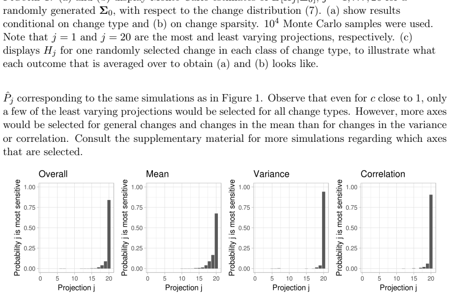
The load-bearing object is the sensitivity of a principal projection: $H_j=H(p_j,q_j)$, the squared Hellinger distance between the marginal densities of $y_{j,t}=v_j^\top x_t$ before and after a change, with post-change parameters drawn from the user-specified change distribution $p(\mu_1,\Sigma_1|\Sigma_0)$. The ranking uses Monte Carlo estimates of $P_j=P(\arg\max_i H_i=j\mid\Sigma_0)$, and the cutoff $c$ controls the chance that the most sensitive projection is omitted. Detection is carried by the corrected mixture log-likelihood statistic $\Lambda^C_{k,t}(p_0)=\sum_{d=1}^{D}\log[1-p_0+p_0\exp\{\ell_{d,k,t}/C(k,t)\}]$ with a Bartlett-type correction $C(k,t)$; applied to the selected standardized projections with $p_0=1$, it yields the stopping rule $T=\inf\{t:\max_k\Lambda^C_{k,t}(1)\ge b\}$, where $b$ is calibrated by a parametric bootstrap that resamples training and monitoring data, incorporating eigenvector estimation uncertainty. For time-dependent data the observations are lag-extended and the bootstrap becomes a nonparametric block bootstrap, giving tailored dynamic PCA.
What would settle it
Fix weak pre-change correlations, $D=100$, $m=200$, and give TPCA a change distribution containing only mean shifts ($p_\mu=1$). Then introduce a sparse variance decrease ($\sigma_d=0.5$ on $2\%$ of streams, remaining correlations unchanged) and compare the expected detection delay of TPCA with that of monitoring the 20 least-varying projections under the same thresholding scheme; if TPCA is far slower while a TPCA prior that also includes variance changes detects it quickly, the claimed automatic tailoring fails under misspecified change priors.
Extended reading notes
Core claim
The central claim is that deliberately choosing low-variance PCA projections, rather than the high-variance ones used for reconstruction, improves online detection of sparse distributional changes. The ranking rule is concrete: for each projection $j$, compute $H_j=H(p_j,q_j)$, the squared Hellinger distance between its marginal normal densities before and after a change drawn from $p(\mu_1,\Sigma_1|\hat\Sigma_0)$; estimate $P_j=P(\arg\max_i H_i=j\mid\Sigma_0)$, the probability that projection $j$ is the single most sensitive one; and keep projections in order of decreasing $P_j$ until their cumulative mass exceeds cutoff $c$. The selected standardized projections are monitored with the corrected mixture log-likelihood statistic $\Lambda^C_{k,t}(1)$, which reduces the full covariance-change problem to detecting marginal mean and variance changes on few streams. Under strong cross-correlation, two least-varying projections suffice to detect the sparsest changes tested ($p=0.02$) with an expected detection delay of 2-3 at false-alarm probability 0.01; on the Tennessee Eastman process, the dynamic version keeps false alarms near nominal and compares favorably with DPCA without a validation set.
Load-bearing premise
The load-bearing premise is that the user's change distribution $p(\mu_1,\Sigma_1|\Sigma_0)$ actually covers the change that occurs; if the true anomaly has a type, size, or sparsity the prior does not include, the projections chosen as most sensitive can be the wrong ones and detection slows or fails.
Editorial extensions
If this is right
- Monitoring the two least-varying projections can reduce dimension by 98% for strongly correlated 100-dimensional streams while detecting sparse mean and variance shifts with an expected detection delay near 2-3 at false-alarm probability 0.01.
- The mixture statistic applied to raw data cannot detect correlation changes, whereas the tailored projection scheme can, extending sparse online detection to the covariance domain.
- Because thresholds are set by bootstrap over regenerated training and monitoring samples, false-alarm control is achieved without a separate large validation set, and the simulation cost scales mainly with the number of selected projections.
- On the Tennessee Eastman process, lag-extending observations and using a nonparametric block bootstrap gives error-controlled dynamic monitoring that beats dynamic PCA (DPCA) on 13 of 20 faults without the validation set DPCA normally relies on.
- The choice of cutoff $c$ between 0.8 and 0.999 changes average expected detection delay very little in the simulations, so the number of projections kept is not a delicate tuning parameter.
Reading between the lines
- As an inference beyond the paper's own claims, the sensitivity of the method to the change prior suggests trying an adaptive change distribution, for example a mixture over change types updated from past alarms or from a small flagged set of historical anomalies.
- The same ranking idea could be transferred to other linear dimension reductions, such as sparse principal components or random projections, whenever the goal is detection rather than reconstruction; the paper notes this direction but does not pursue it.
- On the Tennessee Eastman data the three prior variants perform almost equally, which hints that a uniform change prior may be adequate in complex real processes even when the clean simulations show that the prior type matters.
- A practical diagnostic consequence, left implicit, is that alarms concentrated in the low-variance subspace can be read as evidence of a local, sparse sensor fault rather than a global process shift, aiding post-alarm fault isolation.
Signed reviews
Editorial analysis
A structured set of objections, weighed in public.
Referee Report
Summary. This paper proposes Tailored PCA (TPCA) for online detection of sparse changes in the mean and/or covariance matrix of high-dimensional data. The method first estimates the pre-change correlation matrix from a training sample, then uses Algorithm 1 to simulate B changes from a user-specified change distribution p(µ1, Σ1 | Σ0), computes the Hellinger sensitivity of every principal projection to each simulated change, and selects the minimal subset of projections whose estimated probabilities of being maximally sensitive sum to at least a cutoff c. Monitoring is performed by a mixture generalized log-likelihood statistic applied to the standardized selected projections, with thresholds calibrated by a parametric bootstrap to control the probability of false alarm. The simulation study covers D=100 and D=500, 108 change scenarios, 30 random pre-change correlation matrices, and comparisons with Max/Min PCA and the mixture procedure applied to the raw data. On the Tennessee Eastman Process, a dynamic extension TDPCA with block-bootstrap thresholds is compared with DPCA and Min/Max DPCA. The paper reports that TPCA detects very sparse mean and variance changes almost immediately under high correlation, that a dimension reduction of 80–90% is typical under low correlation, and that TDPCA achieves nominal false-alarm control without a validation set while outperforming DPCA in most fault scenarios once DPCA's false-alarm inflation is accounted for.
Significance. If the claims hold, the paper makes two useful contributions. First, it provides a concrete, implemented answer to the open problem of automatically choosing which PCA projections to monitor for change detection, with code in R packages. Second, it extends the sparse multi-stream monitoring framework to covariance changes and demonstrates finite-sample false-alarm control via bootstrap thresholds without a large validation set. The empirical evaluation is unusually extensive for this literature: 108 change scenarios at D=100 and additional D=500 results, 30 training sets, and a public benchmark with 20 faults. The authors are transparent about the scenarios where the method struggles (weak-correlation variance decreases and sparse correlation changes) and about DPCA's poor false-alarm control. The main weakness is that the tailoring step is evaluated under a prior that is informed of the true change type, leaving the method's central 'automatic tailoring' claim under-tested.
major comments (2)
- [§4.1 and Algorithm 1] The tailoring step in Algorithm 1 requires a user-specified change distribution p(µ1, Σ1 | Σ0), and the central claim that TPCA automatically selects efficient projections is only meaningful if the procedure is robust to plausible misspecification of this distribution. In the main simulation study (§4.1, p. 13) the authors explicitly set pµ = 1 for mean changes, pσ = 1 for variance changes, and pρ = 1 for correlation changes, i.e., the method is told the true change type. Appendix A varies the change-size intervals and whether sizes are equal across affected dimensions, but never varies the type. The bivariate results cited from Tveten (2019, §2) show that the ranking of projections is type-dependent: for a variance decrease, the most varying projection is most sensitive unless the pre-change correlation exceeds about 0.87, whereas mean changes favor the least varying projections. A mean-tailored prior applied to a low-correlation variance-decrease scenario can therefore select projections with low sensitivity. Since the method is proposed as an automatic tailoring tool, the absence of a controlled misspecification study leaves the load-bearing premise untested. I request a simulation study in which the true change type differs from the prior (e.g., mean prior under variance/correlation changes and variance prior under mean changes), reporting EDD and achieved PFA across the same 30 correlation-matrix settings; the TEP comparisons in Section 5 are not a substitute because they involve a single, autocorrelated, non-normal process and the variants TDPCA(mean), TDPCA(var), and TDPCA(unif) are all given the correct fault-type class.
- [§3.3 and Algorithm 2] The bootstrap threshold procedure reuses the projection set J obtained from the original training set when generating each bootstrap replication ('One exception is that J of ˆΣ0 is reused to select projections', §3.3, step 5). The resulting threshold therefore controls the false-alarm probability conditional on the realized J, but not the unconditional PFA that averages over the randomness in J selection. The contribution statement in §1.3 claims the scheme 'includes all sources of estimation uncertainty when finding a threshold'; since J is a random function of the training data, its selection uncertainty is not incorporated. If the intended target is conditional control for the realized training set, this should be stated explicitly and the unconditional claim softened; if unconditional control is intended, the bootstrap should re-run Algorithm 1 inside each replication.
minor comments (6)
- [Section 6] The section header reads 'CONLUDING REMARKS'; it should read 'CONCLUDING REMARKS'.
- [Figures 1, 2, 9-13] Throughout the text and figure captions, '104' and '103' should be typeset as 10^4 and 10^3 to avoid ambiguity.
- [Table 1] In the TPCA column, the entries '0.99 0.995, 0.999' are missing a comma between 0.99 and 0.995.
- [Abstract] The phrase 'based on a criteria' should be 'based on a criterion'.
- [Section 1 and Section 4.1] There are minor typos: 'Additonally' in Section 1 and 'upcomming' in Section 4.1 should be corrected.
- [Figure 3] The caption says 'correlation density plots', but the right-hand panels appear to be histograms; the wording should be clarified or the figures adjusted.
Circularity Check
No significant circularity: the projection-selection step is a disclosed training step, and the reported detection performance is not forced by its inputs.
full rationale
The paper's derivation chain is self-contained. Algorithm 1 explicitly takes a user-specified change distribution p(mu1, Sigma1 | Sigma0) as input and ranks projections by Hellinger sensitivity to draws from that distribution; this is a design/training step, not a hidden prediction. The reported EDD values come from a separate monitoring procedure (mixture GLR, Eqs. 12-13) with bootstrap-calibrated thresholds (Section 3.3), so they are not algebraically forced by the sensitivity ranking. The Section 4.1 disclosure that 'we assumed knowledge about which change type was of interest' is an evaluation limitation: it tests TPCA under a correctly specified change-type prior rather than a misspecified one, but it is explicit and does not make the detection results equivalent to the input by construction. The appendix robustness study varies change size and equal-vs-varying sizes, not change type, so the misspecification question remains open as a robustness/correctness risk, not a circularity. The self-citation to Tveten (2019) supplies a bivariate sensitivity theorem used for motivation, while the high-dimensional algorithm and monitoring results are computed and benchmarked in the present paper and on the external Tennessee Eastman data, including TDPCA(unif) with a non-oracle prior. No specific circular reduction (Eq. X = Eq. Y by construction, or fitted parameter renamed as prediction) can be exhibited.
Assumptions & free parameters
free parameters (5)
- Projection cutoff c =
0.8, 0.9, 0.95, 0.99, 0.995, 0.999 in simulations; 0.9 and 0.99 for TEP
- Change distribution hyperparameters =
Uniform intervals: mean [-1.5, 1.5], std factor [1/2.5, 2.5], correlation factor [0, 1], sparsity K <= D/2, type…
- Window size w =
200
- Mixture sparsity proportion p0 =
0.03, 0.1, 0.3, 1 for the raw-data benchmark; p0=1 for TPCA projections
- Monitoring threshold b =
Calibrated by bootstrap to meet PFA alpha=0.01 at n=100 (or n=kappa-l for TEP)
assumptions (8)
- domain assumption For the clean setup, the data are i.i.d. multivariate normal with unknown mean and covariance under both H0 and H1.
- domain assumption Changes are sparse in the sense that only a subset D of streams changes, with |D| relatively small.
- domain assumption Hellinger distance between marginal distributions of projections is an appropriate sensitivity measure, and selecting projections by probability of being most sensitive is a sound criterion.
- domain assumption The user can specify a change distribution p(mu1, Sigma1 | Sigma0) that represents the changes of interest.
- domain assumption The parametric bootstrap, drawing training and monitoring samples from N(muhat0, Sigmahat0) and reusing the selected J, yields a threshold b that controls the finite-sample PFA.
- domain assumption For the Tennessee Eastman application, lag-extending with l=5 and using a non-parametric block bootstrap adequately accounts for autocorrelation and non-normality.
- standard math Wilks' theorem: 2 times the log-likelihood ratio is asymptotically chi-square with 2 degrees of freedom, used to construct the Bartlett correction in (12).
- standard math Asymptotic normality of sample eigenvectors, Eq. (15) from Muirhead (1982), implying eigenvector estimation variance can be non-negligible.
Cite this review
Pith. "Pith review of Online Detection of Sparse Changes in High-Dimensional Data Streams Using Tailored Projections." pith.science (2026). https://pith.science/paper/OBAI4TI5
@misc{pith2026190802029,
  author       = {Pith},
  title        = {Pith review of: Online Detection of Sparse Changes in High-Dimensional Data Streams Using Tailored Projections},
  year         = {2026},
  howpublished = {\url{https://pith.science/paper/OBAI4TI5}},
  note         = {Machine review of arXiv:1908.02029}
}
read the original abstract
When applying principal component analysis (PCA) for dimension reduction, the most varying projections are usually used in order to retain most of the information. For the purpose of anomaly and change detection, however, the least varying projections are often the most important ones. In this article, we present a novel method that automatically tailors the choice of projections to monitor for sparse changes in the mean and/or covariance matrix of high-dimensional data. A subset of the least varying projections is almost always selected based on a criteria of the projection's sensitivity to changes. Our focus is on online/sequential change detection, where the aim is to detect changes as quickly as possible, while controlling false alarms at a specified level. A combination of tailored PCA and a generalized log-likelihood monitoring procedure displays high efficiency in detecting even very sparse changes in the mean, variance and correlation. We demonstrate on real data that tailored PCA monitoring is efficient for sparse change detection also when the data streams are highly auto-correlated and non-normal. Notably, error control is achieved without a large validation set, which is needed in most existing methods.
Figures


Figures from the paper (10 more)


Reference graph
Works this paper leans on
-
[1]
A likelihood ratio approach to sequential change point detection for a general class of parameters
Banerjee, T., and Veeravalli, V. V. (2015), “Data-Efficient Quickest Change Detection in Sensor Networks,”IEEE Transactions on Signal Processing, 63(14), 3727–3735. Chan, H. P. (2017), “Optimal sequential detection in multi-stream data,”The Annals of Statis- tics, 45(6), 2736–2763. Chan, L.K., andZhang, J.(2001), “CumulativeSumConstrolChartsfortheCovariance...
work page Pith review arXiv 2015
-
[100]
(This is the same figures as shown in the main body of the article, for easier comparison with the figures below.) 103 randomly drawnΣ0’s were used, as well as103 Monte Carlo draws from the change distribution for eachΣ0 Here we present a simulation study for investigating the robustness of our results to change distribution (7), restated below for complete...
work page 2006
Reviewed August 14, 2026 · model on record in the stance chip above.
Discussion (0). Continue with ORCID to comment.