Analysing Global Fixed Income Markets with Tensors

Bruno Scalzo Dees

REVIEW 3 major objections 4 minor 25 references

Analysing Global Fixed Income Markets with Tensors

T0 review · 3 major / 4 minor · reviewed 2026-08-14 · deepseek-v4-flash

Challenge this review Re-run · record.json Download PDF Read on arXiv ↗ Review JSON

Pith's one-line read Global fixed income returns can be modelled as a maturity-by-country tensor whose covariance Kronecker-separates, yielding analytic maturity and country risk factors.

desk verdict A clearly written application of Kronecker-separable covariance to global fixed income, but the paper's empirical 'confirmation' is undercut by its own domestic PCA table. read the letter →

arxiv 1908.02101 v4 pith:UQKGMY5E submitted 2019-08-06 q-fin.PM econ.EMeess.SPq-fin.STstat.AP

Bruno Scalzo Dees This is my paper · ORCID

classification q-fin.PMecon.EMeess.SPq-fin.STstat.AP MSC 91G1091G3062H2515A69

keywords globalfixedincomeKroneckerseparablecovariancetensor-valuedrandomvariablesmultilinearPCAinterestrateswapstermstructurefactorsportfoliohedgingcountryrisk

verification ladder T0 review T1 audit T2 compute T3 formal

The pith

A machine-rendered reading of the paper's core claim, the machinery that carries it, and where it could break.

The reading

This paper argues that the standard flat-view model of international bond risk, which stacks all maturities and countries into one large covariance matrix, discards the natural two-dimensional structure of the data. Instead, weekly returns of fifteen maturities in eight developed economies are arranged as a maturity-by-country matrix $X_t$, and the model assumes its covariance is Kronecker separable: $\Sigma = \sigma^2(\Theta^{(c)}\otimes\Theta^{(m)})$, a scaled product of a maturity covariance density and a country covariance density. That single assumption splits global bond risk into two interpretable factor sets—global level, slope, and curvature within the maturity domain, and a global risk premium plus regional country factors in the country domain. Because the split is analytic, global portfolio optimization and hedging decompose into separate maturity-domain and country-domain problems, reducing the portfolio weight vector from 120 to 23 parameters. On weekly swap data for eight economies from 2015 to 2019, the paper reports that these factors compactly describe the common global macroeconomic environment.

What carries the argument

The load-bearing object is the Kronecker separable covariance decomposition, applied as multilinear PCA to the maturity-by-country return tensor. The identity is $\Sigma=\sigma^2(\Theta^{(c)}\otimes\Theta^{(m)})$ with $\operatorname{tr}(\Theta^{(m)})=\operatorname{tr}(\Theta^{(c)})=1$; $\Theta^{(m)}$ is the average maturity-to-maturity covariance obtained by averaging over country fibres, and $\Theta^{(c)}$ is the average country-to-country covariance obtained by averaging over maturity fibres. Eigendecomposing these two small matrices gives joint eigenvectors $u^{(c)}_k\otimes u^{(m)}_l$ and joint eigenvalues $\lambda^{(c)}_k\lambda^{(m)}_l$, which is the mechanism that turns the intractable full covariance into separate maturity-domain and country-domain portfolio and hedging problems.

What would settle it

Estimate the unrestricted $120\times120$ covariance matrix of the weekly swap returns and test the null hypothesis $\Sigma=\sigma^2(\Theta^{(c)}\otimes\Theta^{(m)})$: compute $\hat\Theta^{(m)}$ from the average of within-country covariance blocks and $\hat\Theta^{(c)}$ from the average of within-maturity covariance blocks, then check whether every cross-country block $\hat\Sigma_{ij}$ is proportional to $\hat\Theta^{(m)}$ with the common factor $\sigma^2\hat\theta^{(c)}_{ij}$ up to sampling error. A likelihood-ratio or residual-norm test that rejects the factorization, or residual blocks whose maturity structure changes from country to country, would falsify the core assumption and with it the separated portfolio and hedging results.

Watch

Extended reading notes

Core claim

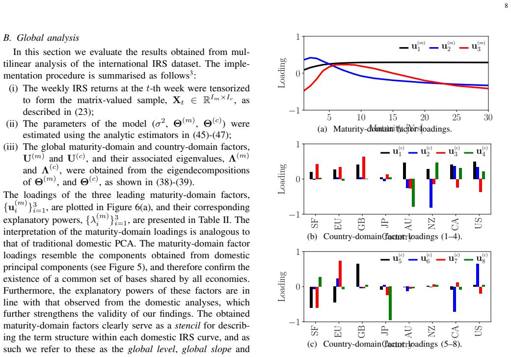
The central claim is that the covariance structure of global fixed income returns is Kronecker separable. For the order-2 tensor $X_t\in\mathbb{R}^{I_m\times I_c}$ of returns arranged by maturity and country, the covariance of $\operatorname{vec}(X_t)$ satisfies $\Sigma=\sigma^2(\Theta^{(c)}\otimes\Theta^{(m)})$, where $\Theta^{(m)}$ and $\Theta^{(c)}$ are unit-trace covariance density matrices describing maturity-to-maturity and country-to-country covariation. Consequently the joint eigenvectors and eigenvalues factor as $U=U^{(c)}\otimes U^{(m)}$ and $\Lambda=\sigma^2(\Lambda^{(c)}\otimes\Lambda^{(m)})$, meaning every country shares the same maturity-domain stencil and every maturity shares the same country-domain stencil. Empirically, the leading maturity-domain factors explain 92.37%, 5.90%, and 0.97% of the variance (global level, slope, and curvature), and the leading country-domain factor, a global risk premium, explains 71.62%, with the remaining country factors separating groups such as (AU, NZ) from the rest. The paper therefore claims that global macro risk in fixed income can be read off these two compact factor sets and used directly for portfolio and hedging decisions.

Load-bearing premise

Everything rests on the assumption that the covariance of global fixed income returns is exactly a Kronecker product of a maturity covariance density and a country covariance density, $\Sigma = \sigma^2(\Theta^{(c)}\otimes\Theta^{(m)})$; the paper introduces this in Section III-B and never compares it with the unrestricted covariance estimated from the same data.

Editorial extensions

If this is right

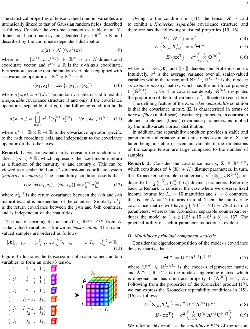
If separability holds, the $120\times120$ covariance of fifteen maturities and eight countries is described by 157 parameters instead of 7260, and the global portfolio weight vector reduces from $I_mI_c=120$ to $I_m+I_c=23$ parameters.
The minimum-variance global portfolio splits into two independent optimizations, one over maturity weights and one over country weights, so the allocation problem can be solved in parallel.
Hedging a long-term bond position requires orthogonality constraints only in the maturity domain, while hedging a domestic position requires constraints only in the country domain, because exposure to a global factor factors as $u^{(c)\top}w^{(c)}\,u^{(m)\top}w^{(m)}$.
The empirical maturity factors reproduce the familiar level, slope, and curvature shape of single-economy term structures, so the model claims that one shared term-structure stencil applies across the eight economies.
The formalism extends to tensors of any order and to other asset classes, so the same separable decomposition can be applied to futures or options with maturity and strike grids.

Reading between the lines

Editorial extensions of the paper, not claims the author makes directly.

The paper does not directly test the Kronecker-separability assumption; a natural extension is to compare the restricted and unrestricted covariance estimates with a likelihood-ratio or residual-norm test, especially in stress periods when factor structures break.
If separability is only approximate, the country-domain loadings can still serve as a data-driven clustering of economies; one could check whether the (AU, NZ) versus rest grouping, or the CA versus US split, is stable across subperiods or tracks currency or trade blocs.
A direct next object is the order-3 tensor of option prices (asset × maturity × strike); the same argument would produce separate asset, maturity, and strike factors of implied-volatility risk, which the paper does not compute.
Because the model forces the maturity factors to be identical across countries, it provides a built-in benchmark for term-structure convergence: large deviations of per-country PCA loadings from the global stencil would indicate exactly where the assumption starts to fail.

Share X Bluesky LinkedIn Reddit HN

Signed reviews

No signed human review yet.

Editorial analysis

A structured set of objections, weighed in public.

Desk editor's note, referee report, and a circularity audit.

Desk Editor's Note

read the letter

The one thing you should know: this paper is a competent exposition of tensor PCA for fixed income, but its main empirical claim outruns the evidence. The math is correct; the untested separability assumption is the whole game.

The application to international IRS markets is the genuinely new piece. The author derives analytic expressions for minimum-variance portfolios and hedging constraints that separate into maturity and country domains, which is a clean consequence of the Kronecker structure and could be practically useful. The paper is clearly written, the estimators are standard, and the parameter reduction from 7260 to 157 is real if the assumption holds.

The problem is that the paper never tests the load-bearing assumption that the global covariance is exactly Kronecker separable. This is not a minor omission. Under the model, every country's domestic covariance block is proportional to the same maturity matrix, so the share of variance explained by the domestic level factor should be identical across countries. Table I shows it ranges from 82% (Japan) to 95% (US), with slope from 3.8% to 14.1%. That spread is far too large to be sampling noise with roughly 200 weekly observations. So the 'global factors' extracted in Section V are eigenvectors of an assumed structure that the data contradict in a direct way. The 'confirmation' is circular: the factors exist by construction once you estimate the mode-wise covariance matrices. There is no goodness-of-fit test, no baseline PCA comparison, no out-of-sample check. The hedging and portfolio results inherit the same fragility.

If the paper were framed as 'under a working separability assumption, here is a useful toolkit,' the derivations stand. As an empirical demonstration of global factors, it does not hold up.

This paper is for practitioners and readers interested in structured covariance models; it gives a clear template but needs a serious empirical overhaul. A referee could usefully push for separability diagnostics and a comparison with flat-view alternatives. I would not reject it outright; it deserves peer review, but conditional on major revision.

Recommendation: send to review, but advise the editor that the empirical claims need heavy revision; treat the abstract's 'confirms' as unsupported.

Referee Report

3 major / 4 minor

Summary. The paper proposes a tensor-valued (Kronecker-separable) covariance model for international fixed income returns. It introduces the separability assumption Σ = σ²(Θ(c)⊗Θ(m)) (Eq. 30), derives maturity-domain and country-domain factors from the eigendecompositions of the mode-specific covariance densities, and uses the decomposition to obtain closed-form minimum-variance portfolios and hedging constraints. An empirical study on weekly IRS data for eight developed economies estimates the model parameters and interprets the leading factors as global level, slope, and curvature in the maturity domain and as country-block factors in the country domain. The paper claims that these results confirm the existence of global risk factors shared by the eight economies.

Significance. If the separability assumption held, the paper would offer a parsimonious and analytically tractable alternative to flat-view PCA, with a large reduction in parameters (Remark 2) and closed-form portfolio and hedging solutions. The tensor algebra exposition is clear, the estimators are simple, and the code is made available, which are concrete strengths. The portfolio and hedging derivations in Section IV are internally consistent given the model. However, the empirical confirmation is not independent: the factors are extracted from the model's own estimated covariance densities, and the paper does not test the key separability assumption or benchmark against an unrestricted PCA. The contribution is therefore methodologically interesting, but the central empirical claim is not yet supported by the evidence presented.

major comments (3)

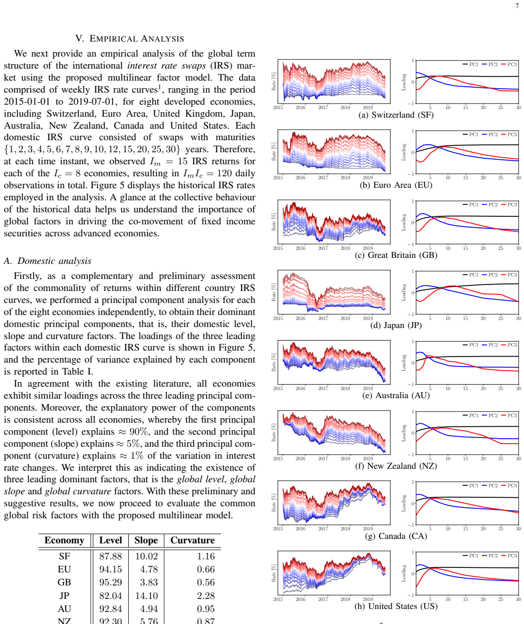
[Section III-B, Eq. (30); Section III-C, Eq. (37); Table I] The Kronecker separability assumption is the load-bearing element of the empirical and portfolio analysis, but it is never tested. Eq. (37) implies that every country's domestic covariance block is proportional to the same Θ(m), so under the model the fractions of variance explained by the domestic level, slope, and curvature components must be equal across countries up to sampling noise. Table I shows the first domestic PC explains 82.04% (JP) to 95.30% (US), the second 3.83% (GB) to 14.10% (JP), and the third 0.47% (US) to 2.28% (JP). This dispersion is large relative to what sampling variation would plausibly produce with weekly data, so the paper's own reported numbers are inconsistent with exact separability. At minimum, the paper should report a goodness-of-fit test for Eq. (30), for example by comparing the separable covariance to the unrestricted sample covariance with an appropriate penalty or cross-validation, and an out-of-sample or bootstrap assessment. Without this, the maturity/country factors in Section V-B cannot be said to represent the actual risk structure.
[Section V-B, Tables II and III] The empirical 'confirmation' is circular in the following sense: the global factors u(m) and u(c) are by construction the eigenvectors of the estimated mode-specific covariance densities Θ(m) and Θ(c) (Eqs. 38–39), so their existence does not require an empirical test. The similarity between the maturity-factor loadings and the domestic PCs (Figure 5 vs Figure 6(a)) is also expected, because Θ(m) is an average of domestic covariance matrices (Eq. 28). The paper should therefore present the empirical analysis as an illustration of the model's output, not as evidence for the existence of global factors. To support the existence claim, the paper would need to show that the separable model outperforms a flat-view PCA baseline, or that its factors have out-of-sample predictive content for the cross-section of returns.
[Section IV, Eqs. (52)–(59)] The portfolio and hedging results are derived from the separable covariance in Eq. (30). Since the assumption is not validated, the practical hedging constraints (e.g., Eq. (56) imposing orthogonality to maturity factors) and the Kronecker-structured minimum-variance portfolio (Eq. (52)) inherit the same unverified restriction. If the data reject separability, the hedging portfolio constructed in the maturity domain alone need not hedge the true factor exposures. The paper should at least demonstrate robustness of the hedging solutions to deviations from separability, or reframe the results as conditional on the model.

minor comments (4)

[Section III-A, Eq. (24)] The definitions of the maturity and country fibres appear reversed: f_i^(m) is defined as the vector of returns across maturities for country i, which is a country fibre, not a maturity fibre, and vice versa. Please clarify the terminology.
[Section V, first paragraph] The phrase 'The data comprised of weekly IRS rate curves' should be 'The data comprised weekly IRS rate curves' or 'The data consisted of weekly IRS rate curves'.
[Section V-A, Table I] The abbreviation 'SF' for Switzerland is used, while the standard code is 'CH' or 'SW'; please define the abbreviation in the table or use a consistent ISO code.
[Section III-E, Eqs. (45)–(47)] The estimators in (45)–(47) are described as maximum likelihood estimators, but no derivation is given. For the Kronecker covariance model in Eq. (30), the maximum likelihood estimator generally requires an iterative procedure, so the closed-form expressions appear to be method-of-moments estimators. Please provide a derivation or amend the claim.

Circularity Check

1 steps flagged · score 6.0 of 10

The abstract's 'confirms the existence of global risk factors' restates the assumed Kronecker-separable covariance rather than testing it.

fitted input called prediction [Sec. III-B Eq. (30); Sec. III-D Eqs. (38)-(39); Sec. V-B steps (ii)-(iii) and confirmation paragraph]
"Σ = σ2(Θ(c)⊗Θ(m)) (30) ... Θ(m) = U(m)Λ(m)U(m)T (38); Θ(c) = U(c)Λ(c)U(c)T (39) ... (ii) The parameters of the model (σ2, Θ(m), Θ(c)) were estimated using the analytic estimators in (45)-(47); (iii) The global maturity-domain and country-domain factors, U(m) and U(c), and their associated eigenvalues, Λ(m) and Λ(c), were obtained from the eigendecompositions of Θ(m), and Θ(c), as shown in (38)-(39). ..."

The 'global maturity-domain factors' are, by construction, the eigenvectors of Θ(m), and Eq. (37) already makes Θ(m) common to every country's domestic covariance block (Σii = σ2θ(c)ii Θ(m)). Estimating Θ(m) via (45)-(47) and diagonalizing it therefore cannot empirically 'confirm' a shared set of bases; the sharing is built into the assumed separable Σ in Eq. (30), not discovered. The only independent evidence is the domestic PCA similarity in Sec. V-A, but the paper's own Table I shows level shares ranging 82.04% (JP) to 95.30% (US) and slope shares 3.83% (GB) to 14.10% (JP), which contradicts the exact proportionality in Eq. (37) unless treated as noise. Thus the abstract's 'confirms the existence of global risk factors' is a fitted input relabelled as a prediction.

full rationale

The paper's model-building is explicit: Section III-B is titled 'Kronecker separability assumptions' and Eq. (30) imposes Σ = σ2(Θ(c)⊗Θ(m)). The maturity- and country-domain factors are formally defined as eigenvectors of the fitted matrices Θ(m) and Θ(c) (Eqs. (38)-(39)), so their derivation is self-contained and not circular in itself. The circularity enters at the empirical-claim level: Section V-B estimates the parameters of that assumed structure and then presents the resulting eigenvectors as a confirmation of common global factors. That is a fitted input called a prediction. The paper does not test separability, and its own Table I provides an internal check that exact separability fails: under Eq. (37) every domestic covariance block must be a scalar multiple of the same Θ(m), so the fractions of variance explained by the first three maturity PCs should be identical across economies; the observed shares vary substantially. Including this internal inconsistency strengthens the verdict that the confirmation claim is not independently supported. The self-citation [16] for tensor-Gaussian properties is not load-bearing because the same standard facts are cited to [15] and are not the source of the circularity; it does not raise the score beyond the fitted-input issue. Because the paper does contain a genuine independent observation (domestic PCA loadings are similar across economies) and the portfolio/hedging algebra is a valid consequence of the stated assumption, the score is 6 rather than 8 or 10.

Assumptions & free parameters 3 free parameters · 3 assumptions · 0 invented entities

The model rests on the untested Kronecker separability assumption plus standard statistical assumptions. The fitted parameters are the covariance densities; no new physical or economic entities are introduced.

free parameters (3)

σ² = estimated from data via Eq. (45)
Average variance scale; fitted to the sample.
Θ(m) = 15×15 matrix estimated via Eq. (46)
Maturity-domain covariance density; its eigendecomposition produces the global level, slope, and curvature factors.
Θ(c) = 8×8 matrix estimated via Eq. (47)
Country-domain covariance density; its eigendecomposition produces country factors.

assumptions (3)

domain assumption Returns xt(m,c) are i.i.d. Gaussian with zero mean (Eq. 22).
Used to justify maximum likelihood estimation, but the central results are likely robust to the Gaussianity; this is a background statistical assumption.
domain assumption The covariance operator is separable: σ(z1,z2) = ∏ σ(n)(z1,z2) (Eq. 11), so Σ = σ²(Θ(c)⊗Θ(m)) (Eq. 30).
This is the load-bearing assumption that yields the factor decomposition; it is not derived or tested in the paper.
domain assumption The estimators (45)-(47) are maximum likelihood and consistent, as cited from the author's own preprint [16].
Relies on a self-cited result for asymptotic properties; no independent verification is provided.

how reviews work

0 comments

Cite this review

Pith. "Pith review of Analysing Global Fixed Income Markets with Tensors." pith.science (2026). https://pith.science/paper/UQKGMY5E

@misc{pith2026190802101,
  author       = {Pith},
  title        = {Pith review of: Analysing Global Fixed Income Markets with Tensors},
  year         = {2026},
  howpublished = {\url{https://pith.science/paper/UQKGMY5E}},
  note         = {Machine review of arXiv:1908.02101}
}

read the original abstract

Global fixed income returns span across multiple maturities and economies, that is, they naturally reside on multi-dimensional data structures referred to as tensors. In contrast to standard "flat-view" multivariate models that are agnostic to data structure and only describe linear pairwise relationships, we introduce a tensor-valued approach to model the global risks shared by multiple interest rate curves. In this way, the estimated risk factors can be analytically decomposed into maturity-domain and country-domain constituents, which allows the investor to devise rigorous and tractable global portfolio management and hedging strategies tailored to each risk domain. An empirical analysis confirms the existence of global risk factors shared by eight developed economies, and demonstrates their ability to compactly describe the global macroeconomic environment.

Figures

Figures reproduced from arXiv: 1908.02101 by the authors.

**Figure 3.** Tensorization of scalar variables on a 3D coordinate [PITH_FULL_IMAGE:figures/full_fig_p003_3.png] view at source ↗

**Figure 4.** Illustration of a tensor-valued sample, represented in () [PITH_FULL_IMAGE:figures/full_fig_p004_4.png] view at source ↗

Figures from the paper (2 more)

**Figure 5.** Figure 5: Weekly swap rates2 for each economy with maturities {1, 2, 3, 4, 5, 6, 7, 8, 9, 10, 12, 15, 20, 25, 30} years (respectively coloured from blue to red) during the period 2015-01-01 to 2019-07-01 (left panel) and their corresponding level, slope and curvature component…

**Figure 6.** Figure 6: Loadings of the three leading maturity-domain global [PITH_FULL_IMAGE:figures/full_fig_p008_6.png]

Discussion (0). Continue with ORCID to comment.

Reference graph

Works this paper leans on

25 extracted references · 25 canonical work pages

[1]

Common Factors Affecting Bond Returns

R. Litterman and J. Scheinkmann, “Common Factors Affecting Bond Returns.” Journal of Fixed Income , vol. 1, pp. 54–61, 1991

work page 1991
[2]

I. T. Jolliffe, Principal Component Analysis . New York: Springer– Verlag, 1986

work page 1986
[3]

Term Structure and V olatility Shocks,

A. P. Rodrigues, “Term Structure and V olatility Shocks,”Working Paper, Federal Reserve Bank of New York , 1997

work page 1997
[4]

Common Factors in Inter- national Bond Returns,

J. Driessen, B. Melenberg, and T. Nijman, “Common Factors in Inter- national Bond Returns,” Journal of International Money and Finance , vol. 22, pp. 629–656, 2003

work page 2003
[5]

Global Term Structure Modeling using Principal Components Analysis,

A. Novosyolov and D. Satchkov, “Global Term Structure Modeling using Principal Components Analysis,” Journal of Asset Management , vol. 9, pp. 49–60, 2008

work page 2008
[6]

Flury, Common Principal Components and Related Multivariate Models

B. Flury, Common Principal Components and Related Multivariate Models. New York: Wiley, 1988

work page 1988
[7]

Common Factors, Principal Components Analysis, and the Term Structure of Interest Rates,

J. Juneja, “Common Factors, Principal Components Analysis, and the Term Structure of Interest Rates,” International Review of Financial Analysis, vol. 24, pp. 48–56, 2012

work page 2012
[8]

An Inter-Battery Method of Factor Analysis,

L. R. Tucker, “An Inter-Battery Method of Factor Analysis,” Psychome- trika, vol. 23, pp. 111–136, 1958

work page 1958

Show all 25 references

[9]

Why Common Factors in Inter- national Bond Returns Are Not so Common,

C. P ´erignon, D. R. Smith, and C. Villa, “Why Common Factors in Inter- national Bond Returns Are Not so Common,” Journal of International Money and Finance, vol. 26, pp. 284–304, 2007

2007
[10]

Tensor Decompositions and Applica- tions,

T. G. Kolda and B. W. Bader, “Tensor Decompositions and Applica- tions,” SIAM Review, vol. 51, no. 3, pp. 455–500, 2009

2009
[11]

Tensor Decompositions for Signal Processing Applications,

A. Cichocki, D. P. Mandic, A. H. Phan, C. F. Caiafa, G. Zhou, Q. Zhao, and L. De Lathauwer, “Tensor Decompositions for Signal Processing Applications,” IEEE Signal Processing Magazine , vol. 145, pp. 145– 163, 2015

2015
[12]

Tensor Networks for Dimensionality Reduction and Large- Scale Optimizations. Part 1: Low–Rank Tensor Decompositions,

A. Cichocki, A. H. Phan, Q. Zhao, N. Lee, I. Oseledets, and D. P. Mandic, “Tensor Networks for Dimensionality Reduction and Large- Scale Optimizations. Part 1: Low–Rank Tensor Decompositions,” Foun- dations and Trends in Machine Learning , vol. 9, no. 4–5, pp. 249–429, 2017

2017
[13]

Tensor Networks for Dimensionality Reduction and Large-Scale Optimizations. Part 2: Applications and Future Perspec- tives,

A. Cichocki, A. H. Phan, Q. Zhao, N. Lee, I. Oseledets, M. Sugiyama, and D. P. Mandic, “Tensor Networks for Dimensionality Reduction and Large-Scale Optimizations. Part 2: Applications and Future Perspec- tives,” Foundations and Trends in Machine Learning , vol. 9, no. 6, pp. ...

2017
[14]

Tensor Decomposition for Signal Processing and Machine Learning,

N. D. Siridopoulos, L. De Lathauwer, X. Fu, K. Huang, E. E. Papalex- akis, and C. Faloutsos, “Tensor Decomposition for Signal Processing and Machine Learning,” IEEE Transactions on Signal Processing , vol. 65, no. 13, pp. 3551–3582, 2017

2017
[15]

Separable Covariance Arrays via the Tucker Product, with Applications to Multivariate Relational Data,

P. D. Hoff, “Separable Covariance Arrays via the Tucker Product, with Applications to Multivariate Relational Data,” Bayesian Analysis, vol. 6, no. 2, pp. 179–196, 2011

2011
[16]

A Statistically Identiﬁable Model for Tensor-Valued Gaussian Random Variables,

B. Scalzo Dees and D. P. Mandic, “A Statistically Identiﬁable Model for Tensor-Valued Gaussian Random Variables,” arXiv:1911.02915, 2019

1911 arXiv
[17]

Matrix Differential Calculus with Applications to Simple, Hadamard, and Kronecker Products,

J. R. Magnus and H. Neudecker, “Matrix Differential Calculus with Applications to Simple, Hadamard, and Kronecker Products,” Journal of Mathematical Psychology , vol. 29, pp. 474–492, 1985

1985
[18]

Some Mathematical Notes on Three-Mode Factor Anal- ysis,

L. R. Tucker, “Some Mathematical Notes on Three-Mode Factor Anal- ysis,” Psychometrika, vol. 31, no. 3, pp. 279–311, 1966

1966
[19]

A Multilinear Singular Value Decomposition,

L. De Lathauwer, B. D. Moor, and J. Vandewalle, “A Multilinear Singular Value Decomposition,” SIAM Journal on Matrix Analysis and Applications, vol. 21, no. 4, pp. 1253–1278, 2000

2000
[20]

N. A. Weiss, P. T. Holmes, and M. Hardy, A Course in Probability . Pearson Addison Wesley, 2005

2005
[21]

Principles of Principal Components: A Fresh Look at Risk, Hedging, and Relative Value,

“Principles of Principal Components: A Fresh Look at Risk, Hedging, and Relative Value,” Research Report, Solomon Smith Barney , 2000

2000
[22]

PCA Unleashed,

“PCA Unleashed,” Research Report, Credit Suisse , 2015

2015
[23]

Introducing a Relative Value Tool for Swaps,

“Introducing a Relative Value Tool for Swaps,” Research Report, Stan- dard Chartered, 2013

2013
[24]

Market Musings – Relative Value Across the U.S. Swap Surface: A PCA Approach,

“Market Musings – Relative Value Across the U.S. Swap Surface: A PCA Approach,” Research Report, TD Securities , 2015

2015
[25]

HOTTBOX: Higher Order Tensor ToolBOX,

I. Kisil, B. Scalzo Dees, A. Moniri, G. G. Calvi, and D. P. Mandic, “HOTTBOX: Higher Order Tensor ToolBOX,” https://hottbox.github.io

Pith tools

Reviewed August 14, 2026 · model on record in the stance chip above.

[1] [1]

Common Factors Affecting Bond Returns

R. Litterman and J. Scheinkmann, “Common Factors Affecting Bond Returns.” Journal of Fixed Income , vol. 1, pp. 54–61, 1991

work page 1991

[2] [2]

I. T. Jolliffe, Principal Component Analysis . New York: Springer– Verlag, 1986

work page 1986

[3] [3]

Term Structure and V olatility Shocks,

A. P. Rodrigues, “Term Structure and V olatility Shocks,”Working Paper, Federal Reserve Bank of New York , 1997

work page 1997

[4] [4]

Common Factors in Inter- national Bond Returns,

J. Driessen, B. Melenberg, and T. Nijman, “Common Factors in Inter- national Bond Returns,” Journal of International Money and Finance , vol. 22, pp. 629–656, 2003

work page 2003

[5] [5]

Global Term Structure Modeling using Principal Components Analysis,

A. Novosyolov and D. Satchkov, “Global Term Structure Modeling using Principal Components Analysis,” Journal of Asset Management , vol. 9, pp. 49–60, 2008

work page 2008

[6] [6]

Flury, Common Principal Components and Related Multivariate Models

B. Flury, Common Principal Components and Related Multivariate Models. New York: Wiley, 1988

work page 1988

[7] [7]

Common Factors, Principal Components Analysis, and the Term Structure of Interest Rates,

J. Juneja, “Common Factors, Principal Components Analysis, and the Term Structure of Interest Rates,” International Review of Financial Analysis, vol. 24, pp. 48–56, 2012

work page 2012

[8] [8]

An Inter-Battery Method of Factor Analysis,

L. R. Tucker, “An Inter-Battery Method of Factor Analysis,” Psychome- trika, vol. 23, pp. 111–136, 1958

work page 1958