REVIEW 4 major objections 5 minor 46 references
Photo-acoustic tomographic image reconstruction from reduced data using physically inspired regularization
T0 review · 4 major / 5 minor · reviewed 2026-08-14 · deepseek-v4-flash
Pith's one-line read Joint sparsity prior lifts limited-data PAT reconstruction quality
desk verdict A promising limited-data PAT reconstruction method with a useful matrix-free implementation, but the physical prior is asserted rather than demonstrated and the paper needs an ablation. read the letter →
The pith
A machine-rendered reading of the paper's core claim, the machinery that carries it, and where it could break.
The reading
What carries the argument
The central object is a non-convex regularizer that couples pixel intensity to second-order derivatives. The first form is $$R_{h,1}(p_0,q)=\sum_r \left(\epsilon+\$\alpha$(p_0)$_r^{2}$+(1-\$\alpha$)\sum_i (D_{2,i}p_0)$_r^{2}$\right)^q$$ with $q<0.5$; the second form separates the intensity and derivative terms before raising each to the power $q$. The fractional power $q$ is what makes the cost non-convex, and the graduated non-convexity outer loop starts at the convex value $q=0.5$ and decreases $q$ toward $0.25$, warm-starting each inner solve. The inner solver is a preconditioned gradient method whose preconditioner approximates a damped Newton step and is applied with conjugate gradients. Memory is controlled by a matrix-free forward model that uses the exact time-propagator relation $p(r,t)=\mathcal{F}^{-1}\{\hat{P}_0(k)\cos(c_0\|k\|t)\}$, so the operator $H^T H$ is applied as a sequence of Fourier multiplications rather than stored as a matrix.
What would settle it
Take an unseen class of PAT images, for example vascular or organ images with diffuse backgrounds, and compute the joint histogram of pixel intensity against second-derivative magnitude; if the high-intensity, high-derivative pixels are not markedly sparser than in generic images, the proposed method should fail to beat the FISTA baseline at 16–32 transducers. A complementary check is to rerun the 16-transducer experiments with the GNC loop disabled and $q$ fixed at 0.25; if artifacts return, the convergence schedule rather than the prior is doing the work.
Extended reading notes
Core claim
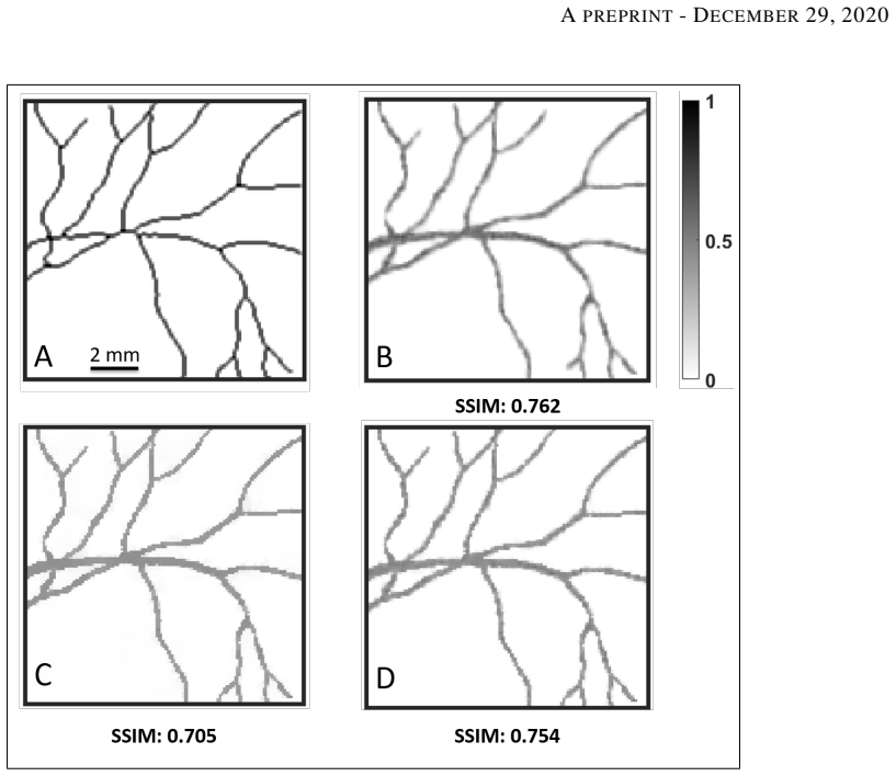
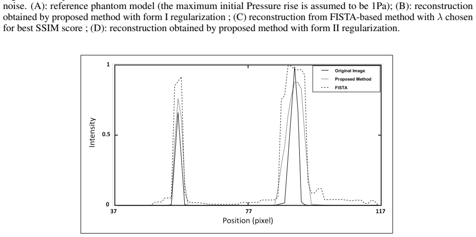
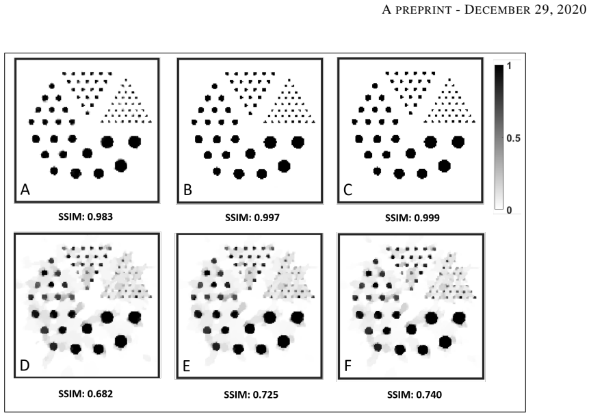
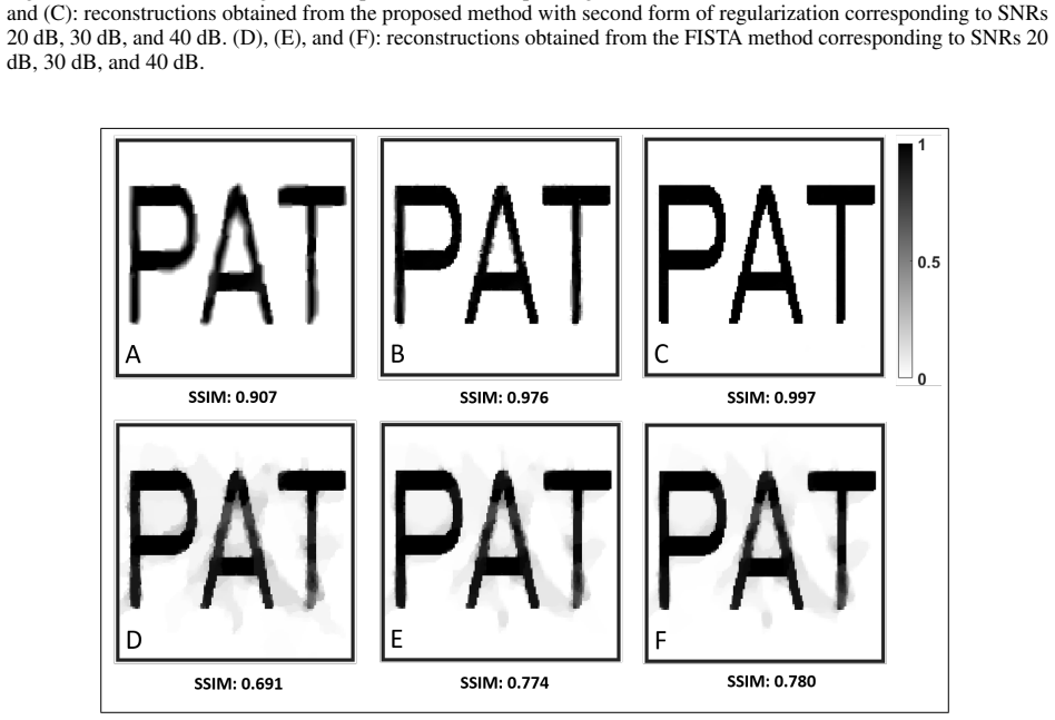
The paper's central claim is that a reconstruction prior designed around the physical structure of photoacoustic images, rather than a generic image prior, can recover accurate initial-pressure distributions from a fraction of the measurements normally required. Concretely, the authors assert that in PAT images high intensity and high second-order derivatives are jointly sparse, and that a regularizer encoding this joint sparsity, minimized by their custom graduated non-convex solver, produces higher SSIM and FOM scores than the FISTA-based total-variation baseline in all tested scenarios: 16, 32, 64, and 128 transducers at 20, 30, and 40 dB input noise, plus real horsehair-phantom data. The largest reported gains occur at 16–32 transducers, where the baseline reconstructions degrade visibly while the proposed method remains close to full-array quality.
Load-bearing premise
The load-bearing premise is the asserted structural property that in photoacoustic images bright pixels and pixels with large second-order derivatives tend to occupy the same sparse locations, a claim the paper supports by observation rather than quantitative statistics; if that property is absent for a given image class, the regularizer's advantage over generic total variation would disappear.
Editorial extensions
If this is right
- PAT systems could use 16 or 32 transducers instead of 128 and still recover images close to full-array quality, which would shorten scan times and lower equipment cost.
- The advantage persists from 20 dB to 40 dB input noise, and the largest margins occur at low SNR, so the method is useful where measurements are noisy or laser fluence is limited.
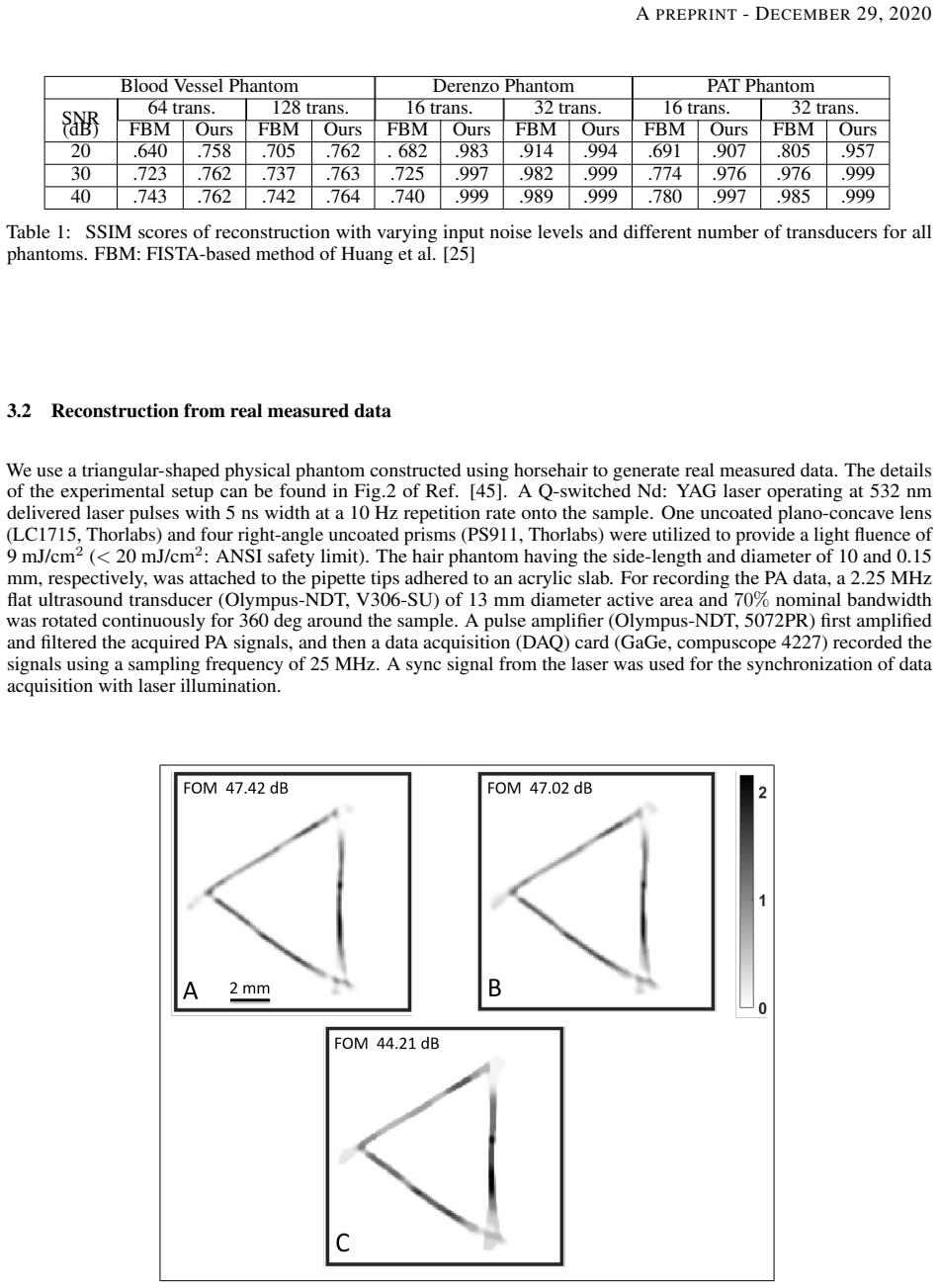
- The real horsehair-phantom test gives roughly a 3 dB improvement in the peak-to-noise figure of merit over the FISTA baseline, indicating the benefit survives experimental transducer-response and setup effects.
- Because the second regularizer form performs better on some phantoms and the first on others, the paper gives users a practical choice rather than a single fixed prior.
Reading between the lines
- Extending the joint-sparsity idea beyond PAT, the same regularizer could transfer to other high-contrast tomographic modalities such as fluorescence microscopy or diffuse optical tomography, where bright structures and sharp boundaries are also sparse.
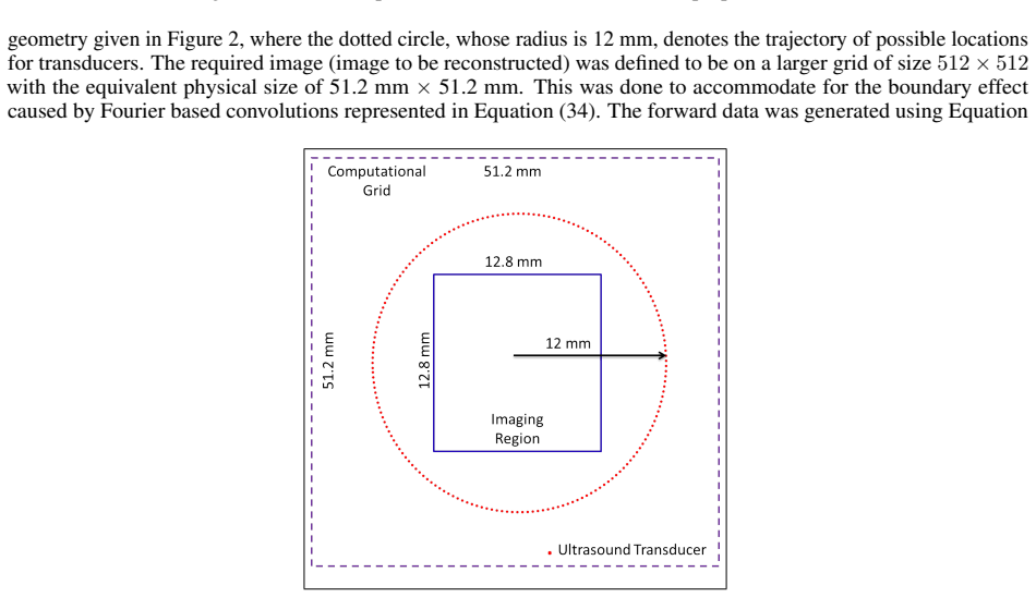
- A consequence the paper does not develop: the matrix-free Fourier-cosine propagator assumes a homogeneous, lossless acoustic medium and transducer positions on the imaging grid, so adapting it to heterogeneous sound speed or arbitrary detector layouts would need a different fast propagator and would likely reduce the memory savings.
- The reported parameter settings ($q=0.25$, $n_s=10$, $\alpha=0.5$, $\lambda_p=10\lambda$) were chosen as adequate across the tested cases, so a broader tuning study on unseen anatomies and noise levels would show whether the SSIM margins, especially the large gap at 16 transducers, persist or shrink.
- The SSIM curves suggest an adaptive acquisition strategy: add transducer positions only until the reconstruction quality plateaus, rather than always using a fixed large array.
Signed reviews
Editorial analysis
A structured set of objections, weighed in public.
Referee Report
Summary. The paper proposes a model-based photoacoustic tomography (PAT) reconstruction method for reduced-size datasets. The key novelty is a non-convex regularizer that couples image intensity with second-order derivatives, motivated by an asserted 'joint sparsity' property of PAT images (Section 2.1, Eqs. 13-14). The authors develop a preconditioned gradient algorithm with graduated non-convexity (GNC) for the resulting non-convex problem, and derive a matrix-free implementation of the PAT forward model based on a Fourier-domain time propagator (Section 2.4, Eq. 34). The method is evaluated on three simulated phantoms (blood vessel, Derenzo, PAT) at 16-128 transducers and 20-40 dB noise, plus one real horsehair phantom, comparing against a FISTA-based total-variation method by Huang et al. Reported SSIM and FOM gains favor the proposed method, especially at very limited transducer counts.
Significance. If the reported gains hold, the paper contributes a practical reconstruction method for limited-data PAT, with the matrix-free forward-model implementation being a genuinely useful engineering contribution that removes a memory bottleneck for large images. The comparison across transducer counts and noise levels is reasonably extensive, and the inclusion of real measured data strengthens the claims. However, the conceptual novelty—the joint-sparsity prior—is asserted rather than demonstrated. Because the regularizer changes derivative order, convexity, and intensity-derivative coupling simultaneously, the current evidence does not establish that the physical prior is the cause of the improvements. The paper would be significantly strengthened by a controlled ablation and by specifying the parameter-selection protocol, particularly for the regularization weight, to ensure a fair comparison. The central idea is defensible, but the evidence as presented is not yet conclusive on the mechanism.
major comments (4)
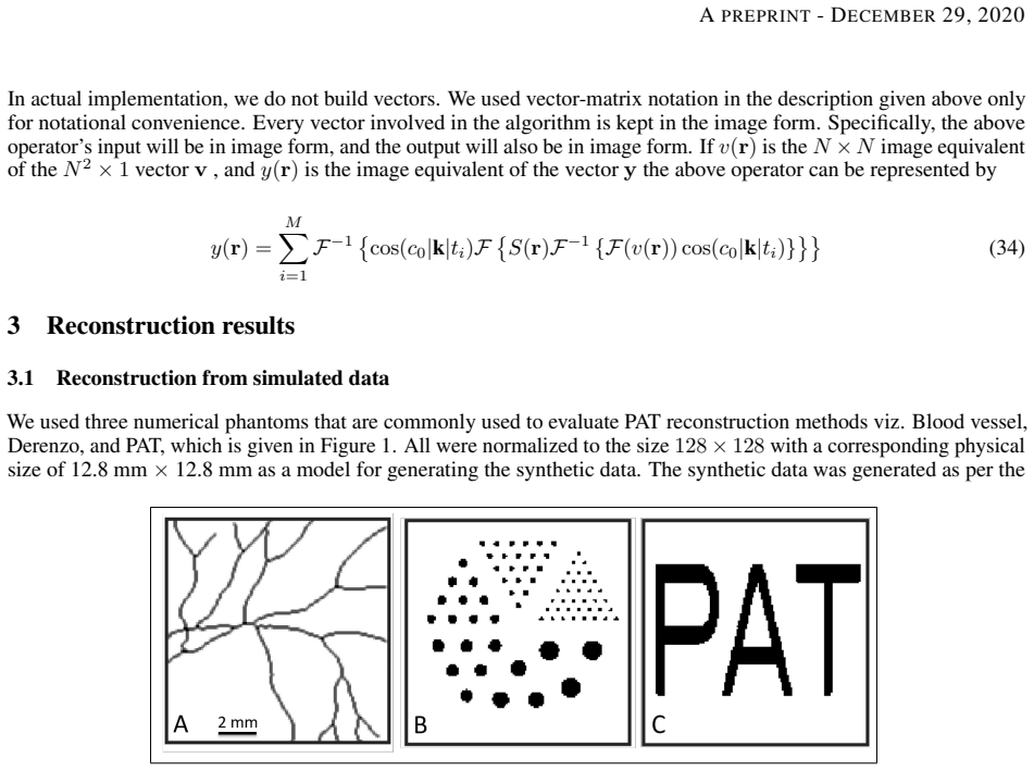
- [Section 2.1; Eqs. (13)-(14)] The paper's central claim is that PAT images exhibit joint sparsity of high intensities and high second-order derivatives, and that this prior is responsible for the reconstruction gains. However, this property is only asserted ('we observe' in Section 2.1) without any quantitative evidence. No histograms, scatter plots, or statistical tests are provided to show that PAT images have this structure beyond what generic first-order or second-order smoothness priors would capture. Since the regularizer is specifically designed around this property, the reader cannot verify the premise. Please add quantitative evidence of the joint-sparsity property for the phantoms and real PAT images used, and discuss whether it holds for other PAT image classes (e.g., vasculature versus diffuse absorption).
- [Section 3.1; Table 1] There is no controlled ablation that isolates the proposed joint-sparsity mechanism. The proposed cost (Eq. 13) differs from the FISTA/TV-1 baseline along three axes simultaneously: second-order versus first-order derivatives, non-convexity with q=0.25 solved by GNC, and intensity-derivative coupling through α. The reported SSIM gains (Table 1) could therefore be caused entirely by higher-order smoothness, by non-convex regularization, or by the specific optimization procedure, rather than by the physical prior. Please include at least the following ablations: (i) α=0 and α=1 in Eq. (13), (ii) a convex control with q=0.5 in the same GNC framework, and (iii) a second-order TV or TGV baseline. Without these, the abstract's and conclusions' attribution of improvements to the joint-sparsity prior is not supported.
- [Section 3.1; parameter selection] The selection of the regularization parameter λ is described only as 'determined using the model itself' (Section 3.1), which is not a reproducible or falsifiable protocol. In contrast, the FISTA baseline is explicitly tuned for best SSIM ('λ chosen for best SSIM score' in Figures 3-7). If the proposed method's λ is chosen by a different criterion or by visual inspection, the comparison may be biased in its favor. Please specify the exact λ-selection procedure for both methods, and ideally use an identical criterion (e.g., best SSIM on a validation set, or a principled discrepancy principle) for both.
- [Section 2.2; Eq. (17)-(18)] The use of a fixed positivity penalty with λp = 10λ is justified only by 'a series of reconstruction trials' (Section 2.2). This is an ad hoc choice that may not transfer to other phantoms, noise levels, or transducer geometries. Since the positivity constraint is part of the model (Eq. 15), the sensitivity of the results to λp should be reported, or the penalty should be systematically set (e.g., via continuation). Otherwise, the reader cannot assess whether the reported gains are contingent on a manually tuned parameter.
minor comments (5)
- [Section 3.1; runtime] The paper reports that the proposed method takes about 38 minutes per reconstruction versus 30 minutes for FISTA on the same machine, but provides no iteration counts, convergence curves, or memory usage measurements. A brief table of computational cost (iterations, CG calls, memory footprint with the matrix-free implementation) would make the engineering contribution of Section 2.4 concrete.
- [Section 3.1; Figures 6-7] Figures 6 and 7 appear to show the same experiment (16 transducers, three noise levels) for different phantoms, but the captions do not specify which phantom is in each figure. Please make the captions explicit (e.g., 'PAT phantom' and 'Derenzo phantom').
- [Section 3.2; Eq. (35)] The FOM defined in Eq. (35) is computed as 20*log10(S/n), where n is the standard deviation of the 'intensity' of the reconstructed image. It is unclear whether n is computed over the whole image or over a background region. Since the FOM comparison is the only quantitative metric for the real-data experiment, please define the region of interest and the noise estimation method explicitly.
- [Section 2.3; Algorithm 3] The GNC schedule sets q_m = 0.5 - m(0.5-q)/ns, but the text does not describe how the choice of q=0.25 and ns=10 interacts with the line-search tolerances. A sentence explaining the robustness of the GNC schedule to the inner tolerances (as claimed) would help, since Algorithm 3 is central to the non-convex optimization.
- [Section 2.4; Eq. (34)] The matrix-free formula in Eq. (34) is a useful contribution, but the derivation assumes transducers located on image grid points. For the real-data experiment, the transducer is rotated continuously; please clarify how the discrete transducer positions are mapped to grid points, or how the formula is adapted for off-grid positions.
Circularity Check
No circular derivation: the joint-sparsity regularizer is proposed and tested, not fitted or relabeled as a prediction; the minor self-citation is not load-bearing.
full rationale
The paper's derivation chain consists of (i) asserting, not deriving, that PAT images have jointly sparse intensities and second-order derivatives; (ii) constructing the nonconvex regularizer in Eqs. (13)-(14) as a modification of Ref. [34]; (iii) deriving the gradient, preconditioned CG, and GNC optimization; and (iv) evaluating on simulated and real data. No equation in this chain is equivalent by construction to a measured quantity that is then called a prediction. The regularization parameters (alpha=0.5, q=0.25, lambda via the model) are user-selected hyperparameters, not fitted values renamed as outputs. The only self-citation, Ref. [34], supplies the original log-based fluorescence regularizer and the observation that the same sparsity pattern occurs in fluorescence images; the present paper explicitly modifies the log to a fractional power and tests the modified regularizer on PAT data, so the central claim does not reduce to that citation. The simulated-data validation uses the same Fourier-cosine propagator (Eq. (4)) to generate and reconstruct data, which is an inverse-crime-style limitation, but this is a benchmarking weakness, not a circular derivation; the real measured-data experiment provides independent evidence. The main load-bearing scientific weakness is that the asserted joint-sparsity property is supported only by visual assertion and no ablation isolates the proposed prior from second-order smoothness or nonconvexity; that is an evidence gap, not a self-referential reduction. Accordingly, no circular step is identified.
Assumptions & free parameters
free parameters (5)
- lambda (regularization weight) =
not stated; determined using the model itself (Sec. 3.1)
- q (sparsity index) =
0.25
- alpha (relative penalization) =
0.5
- lambda_p (positivity penalty weight) =
10 times lambda
- ns (number of GNC steps) =
10
assumptions (5)
- domain assumption 2D homogeneous, lossless, non-dispersive acoustic medium with point detectors
- domain assumption Photoacoustic source is approximated as H(r)delta(t) under stress and thermal confinement
- domain assumption PAT images have jointly sparse high intensity and high second-order derivatives
- domain assumption Transducers lie on image grid points and sample pressure at points
- ad hoc to paper Quadratic penalty with lambda_p = 10 lambda suffices to enforce non-negativity
Cite this review
Pith. "Pith review of Photo-acoustic tomographic image reconstruction from reduced data using physically inspired regularization." pith.science (2026). https://pith.science/paper/YFGEZGVX
@misc{pith2026190802313,
  author       = {Pith},
  title        = {Pith review of: Photo-acoustic tomographic image reconstruction from reduced data using physically inspired regularization},
  year         = {2026},
  howpublished = {\url{https://pith.science/paper/YFGEZGVX}},
  note         = {Machine review of arXiv:1908.02313}
}
read the original abstract
We propose a model-based image reconstruction method for photoacoustic tomography(PAT) involving a novel form of regularization and demonstrate its ability to recover good quality images from significantly reduced size datasets. The regularization is constructed to suit the physical structure of typical PAT images. We construct it by combining second-order derivatives and intensity into a non-convex form to exploit a structural property of PAT images that we observe: in PAT images, high intensities and high second-order derivatives are jointly sparse. The specific form of regularization constructed here is a modification of the form proposed for fluorescence image restoration. This regularization is combined with a data fidelity cost, and the required image is obtained as the minimizer of this cost. As this regularization is non-convex, the efficiency of the minimization method is crucial in obtaining artifact-free reconstructions. We develop a custom minimization method for efficiently handling this non-convex minimization problem. Further, as non-convex minimization requires a large number of iterations and the PAT forward model in the data-fidelity term has to be applied in the iterations, we propose a computational structure for efficient implementation of the forward model with reduced memory requirements. We evaluate the proposed method on both simulated and real measured data sets and compare them with a recent reconstruction method that is based on a well-known fast iterative shrinkage threshold algorithm (FISTA).
Figures
Figures from the paper (6 more)


Reference graph
Works this paper leans on
-
[1]
Wang L V and Yao J 2016 Nature methods 13 627
work page 2016
-
[2]
Pramanik M, Ku G, Li C and Wang L V 2008 Medical physics 35 2218–2223
work page 2008
-
[3]
Beard P 2011 Interface focus 1 602–631
work page 2011
-
[4]
Zhou Y , Yao J and Wang L V 2016Journal of biomedical optics 21 061007
-
[5]
Upputuri P K and Pramanik M 2016 Journal of Biomedical Optics 22 041006
work page 2016
-
[6]
2017 Nature biomedical engineering 1 0071
Li L, Zhu L, Ma C, Lin L, Yao J, Wang L, Maslov K, Zhang R, Chen W, Shi J et al. 2017 Nature biomedical engineering 1 0071
work page 2017
-
[7]
Han Y , Ding L, Ben X L D, Razansky D, Prakash J and Ntziachristos V 2017Opt. Lett. 42 979–982
-
[8]
Rosenthal A, Ntziachristos V and Razansky D 2013 Current medical imaging reviews 9 318–336
work page 2013
Show all 46 references
-
[9]
Finch D and Patch S K 2004 SIAM journal on mathematical analysis 35 1213–1240
2004
-
[10]
Kunyansky L A 2007 Inverse problems 23 373
2007
-
[11]
Xu M and Wang L V 2002 IEEE transactions on medical imaging 21 814–822
2002
-
[12]
Xu M and Wang L V 2005 Physical Review E 71 016706
2005
-
[13]
Kalva S K and Pramanik M 2016 Journal of Biomedical Optics 21 086011
2016
-
[14]
Pramanik M 2014 JOSA A 31 621–627
2014
-
[15]
Xu Y and Wang L V 2004 Physical review letters 92 033902
2004
-
[16]
Burgholzer P, Matt G J, Haltmeier M and Paltauf G 2007 Physical Review E 75 046706
2007
-
[17]
Treeby B E, Zhang E Z and Cox B T 2010 Inverse Problems 26 115003
2010
-
[18]
Hristova Y , Kuchment P and Nguyen L 2008Inverse Problems 24 055006
-
[19]
Xu Y , Wang L V , Ambartsoumian G and Kuchment P 2004Medical physics 31 724–733
-
[20]
Arridge S, Beard P, Betcke M, Cox B, Huynh N, Lucka F, Ogunlade O and Zhang E 2016Physics in Medicine & Biology 61 8908 14 A PREPRINT - D ECEMBER 29, 2020
2020
-
[21]
Buehler A, Rosenthal A, Jetzfellner T, Dima A, Razansky D and Ntziachristos V 2011 Medical physics 38 1694–1704
2011
-
[22]
Paltauf G, Viator J, Prahl S and Jacques S 2002 The Journal of the Acoustical Society of America 112 1536–1544
2002
-
[23]
Schwab J, Pereverzyev Jr S and Haltmeier M 2018 SIAM Journal on Numerical Analysis 56 160–184
2018
-
[24]
Prakash J, Mandal S, Razansky D and Ntziachristos V 2019 IEEE Transactions on Biomedical Engineering 1–1 ISSN 0018-9294
2019
-
[25]
Huang C, Wang K, Nie L, Wang L V and Anastasio M A 2013 IEEE Transactions on Medical Imaging 32 1097–1110
2013
-
[26]
Arridge S R, Betcke M M, Cox B T, Lucka F and Treeby B E 2016 Inverse Problems 32 115012
2016
-
[27]
Boink Y E, Lagerwerf M J, Steenbergen W, van Gils S A, Manohar S and Brune C 2018Physics in Medicine & Biology 63 045018
-
[28]
Saratoon T, Tarvainen T, Cox B and Arridge S 2013 Inverse Problems 29 075006
2013
-
[29]
Han Y , Tzoumas S, Nunes A, Ntziachristos V and Rosenthal A 2015Medical physics 42 5444–5452
-
[30]
Wang K, Huang C, Kao Y J, Chou C Y , Oraevsky A A and Anastasio M A 2013Medical physics 40
-
[31]
Rosenthal A, Razansky D and Ntziachristos V 2010 IEEE transactions on medical imaging 29 1275–1285
2010
-
[32]
Rosenthal A, Jetzfellner T, Razansky D and Ntziachristos V 2012 IEEE transactions on medical imaging 31 1346–1357
2012
-
[33]
Liu H, Wang K, Peng D, Li H, Zhu Y , Zhang S, Liu M and Tian J 2016IEEE transactions on medical imaging 35 2546–2557
-
[34]
Arigovindan M, Fung J C, Elnatan D, Mennella V , Chan Y H M, Pollard M, Branlund E, Sedat J W and Agard D A 2013 Proceedings of the National Academy of Sciences 201315675
2013
-
[35]
Cox B T, Kara S, Arridge S R and Beard P C 2007 The Journal of the Acoustical Society of America 121 3453–3464
2007
-
[36]
Cox B and Beard P 2005 The Journal of the Acoustical Society of America 117 3616–3627
2005
-
[37]
Xu M and Wang L V 2006 Review of scientific instruments 77 041101
2006
-
[38]
Wang K, Ermilov S A, Su R, Brecht H P, Oraevsky A A and Anastasio M A 2011IEEE transactions on medical imaging 30 203–214
-
[39]
Wang K, Su R, Oraevsky A A and Anastasio M A 2012 Physics in Medicine & Biology 57 5399
2012
-
[40]
Tao M, Yang J and He B 2009 TR0918, Department of Mathematics, Nanjing University
2009
-
[41]
Wang Y , Yang J, Yin W and Zhang Y 2008SIAM Journal on Imaging Sciences 1 248–272
-
[42]
Skariah D G and Arigovindan M 2017 IEEE Transactions on Image Processing 26 4471–4482
2017
-
[43]
Nikolova M, Ng M K and Tam C 2010 IEEE Transactions on Image Processing 19 3073–3088
2010
-
[44]
Zhou Wang, Bovik A C, Sheikh H R and Simoncelli E P 2004 IEEE Transactions on Image Processing 13 600–612
2004
-
[45]
Awasthi N, Kalva S K, Pramanik M and Yalavarthy P K 2018 Journal of Biomedical Optics 23 091413
2018
-
[46]
Li L, Zhu L, Shen Y and Wang L V 2017 Journal of biomedical optics 22 076017 15
2017
Reviewed August 14, 2026 · model on record in the stance chip above.
Discussion (0). Continue with ORCID to comment.