REVIEW 3 major objections 6 minor 24 references
Efficient and robust evaluation of fast particle losses in non-axisymmetric tokamak plasmas
T0 review · 3 major / 6 minor · reviewed 2026-08-14 · deepseek-v4-flash
Pith's one-line read Fast-particle losses in non-axisymmetric tokamak plasmas can be reproduced by a one-dimensional advection-diffusion model whose coefficients come from short orbit-following runs, cutting scan cost a hundredfold.
desk verdict Loss maps are genuinely useful and the advection-diffusion idea is promising, but the coefficients are validated with the same orbit-following code used to make them, and the missing sensitivity analysis leaves the 100x speedup claim undermoored. read the letter →
The pith
A machine-rendered reading of the paper's core claim, the machinery that carries it, and where it could break.
The reading
What carries the argument
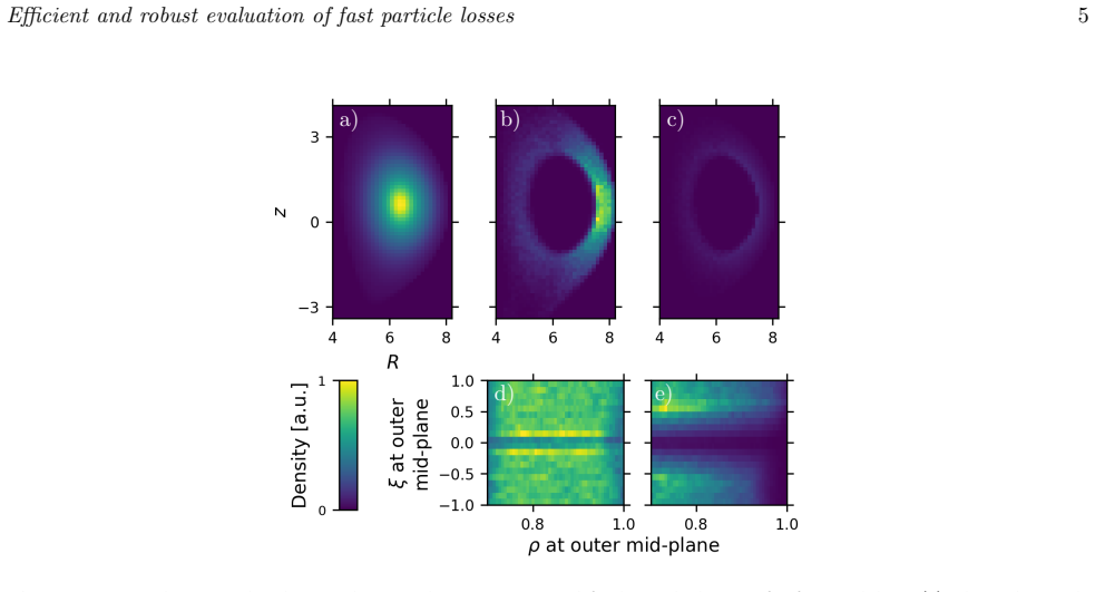
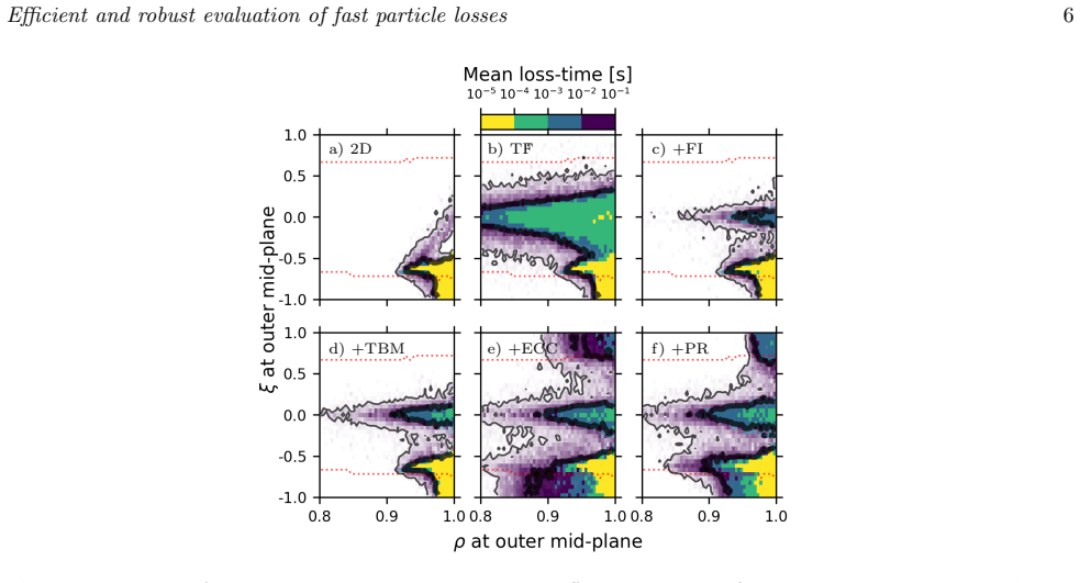
The load-bearing object is the loss map: a histogram of lost-particle fraction in $(\rho',\xi')$ space, where $\rho'$ is the normalized poloidal flux at the outer mid-plane crossing and $\xi'$ is the pitch there. Because every orbit's topology is fixed by these two coordinates at fixed energy, loss channels appear as separated regions identifiable with known mechanisms. The second mechanism is a coefficient-estimation recipe for the advection-diffusion equation $$\frac{\partial f}{\partial t}=-\frac{\partial}{\partial\rho'}(Kf)+\frac{\$partial^{2}$}{\partial{\rho'}^2}(Df),$$ using short orbit-following data: Gaussian displacement statistics for confined markers and inverse-Gaussian first-passage times for lost markers. The loss map supplies both the diagnostic that validates the model and the weighting that lets transport coefficients be evaluated only where transport actually occurs.
What would settle it
Follow a collisionless orbit ensemble in a field with strong stochastic-ripple transport and test whether the radial displacement has Gaussian statistics with variance growing linearly in time and whether loss times follow the inverse-Gaussian distribution; if the inferred coefficients depend on the averaging window $N$ or on the toroidal launch phase of otherwise identical markers, the Markovian one-dimensional description is wrong. A concrete target is the paper's own 16-37\% disagreement: a case where that gap grows with simulation time rather than staying bounded would show the model is not a reliable predictor for that regime.
Extended reading notes
Core claim
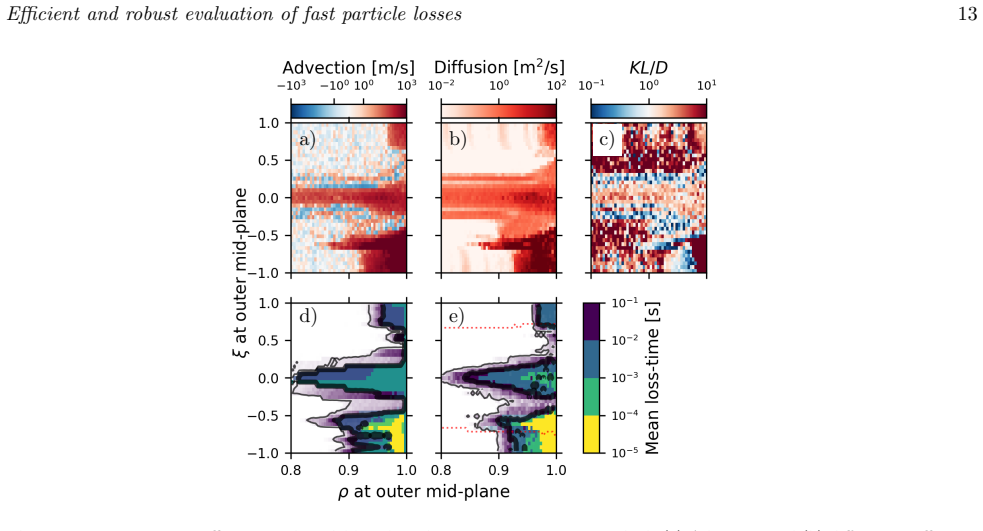
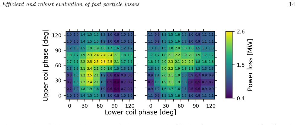
The central claim is that collisionless fast ion transport in a three-dimensional perturbed magnetic field can be modelled to good accuracy as a one-dimensional Fokker-Planck process in the radial coordinate $\rho'$ (flux-surface coordinate at the outer mid-plane), with magnetic moment $\mu$ and energy $E$ treated as parameters. The advection coefficient $K(\rho';\mu,E)$ and diffusion coefficient $D(\rho';\mu,E)$ are not derived from first principles but measured from a very short orbit-following simulation, about a millisecond in these test cases, in which markers are followed for only tens of poloidal orbits. Confined markers yield $K$ and $D$ from the mean and variance of the radial displacement after averaging over ten outer mid-plane crossings; lost markers contribute through the inverse-Gaussian distribution of first-passage times. In the benchmark with the most complete magnetic field, the model predicted 2.46 MW of total lost $\alpha$ power against 1.79 MW from the collisionless full-orbit simulation (1.42 MW versus 1.22 MW when only collisionless-time-scale losses are counted), and the $8\times8$ scan over ELM control coil phases reproduced the two high-loss bands and their crossing point at one hundredth of the computational cost.
Load-bearing premise
The load-bearing premise is that collisionless radial transport is Markovian and local, so that a particle's random walk in $\rho'$ is fully described by one advection and one diffusion coefficient at each point; if the motion has memory, depends on toroidal or poloidal phase, or needs more than two coefficients, the model fails.
Editorial extensions
If this is right
- ELM control coil phase scans that would normally require millions of markers per configuration can be reduced to short coefficient runs plus a cheap one-dimensional solve, making it practical to map the full parameter space of coil phases and currents.
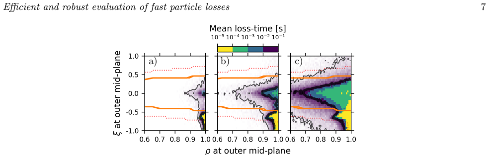
- Because loss maps can be projected from magnetic field structure alone, one can cross-check an orbit-following result or estimate losses without running a dedicated simulation.
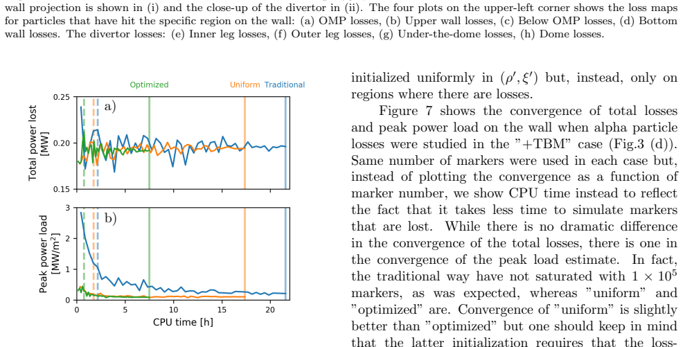
- Marker initialization can be concentrated on the loss channels identified in the map, so peak power load estimates converge with one or two orders of magnitude fewer markers.
- Orbit-averaged transport codes can incorporate three-dimensional-field fast-ion transport by adding the measured advection and diffusion coefficients rather than following orbits in full geometry.
- The collisionless approximation captures most alpha losses at birth energy, so collisions matter mainly near thermal energies where neoclassical transport takes over.
Reading between the lines
- Beyond the paper, the same coefficient-measurement recipe could be applied to runaway electrons or other fast species; the one-dimensional Markov assumption is most plausible for strongly passing populations and would need re-testing there.
- Beyond the paper, if transport coefficients could be estimated from magnetic-field-based projections rather than short orbit runs, the approach might eventually skip orbit-following entirely, although the field-based loss-map projections shown here are close but not yet accurate enough for that.
- Beyond the paper, the systematic overestimate of lost power in the benchmark suggests the model may be collapsing several mechanisms into a single effective diffusion coefficient; checking whether the inferred coefficients are independent of the averaging window and simulation time would test whether the Markov description is genuinely valid.
Signed reviews
Editorial analysis
A structured set of objections, weighed in public.
Referee Report
Summary. The paper introduces and demonstrates loss-map techniques for fast-particle loss studies in non-axisymmetric tokamaks, applied mainly to ITER. The loss map is a representation of particle birth location in (rho-prime, xi-prime) space that allows loss channels (first-orbit, ripple-induced, stochastic field-line, perturbed banana) to be identified and connected to magnetic field structure. The paper presents optimized marker initialization for improved convergence of total and peak power loads, magnetic-field-based projections for estimating losses without orbit-following, and an analysis of collisional effects. The central new claim is that collisionless fast-ion transport can be described as a one-dimensional advection-diffusion process with coefficients K(rho',mu,E) and D(rho',mu,E) evaluated from a short (1 ms) orbit-following simulation, and that the resulting model can replace full slowing-down simulations for parameter scans, specifically a 64-case ELM control coil phase scan that is claimed to be 100 times faster than full simulations while reproducing the overall loss landscape.
Significance. If the central claim holds, the advection-diffusion model would be a practically useful tool for fast design scans of fast-ion losses, a problem of direct relevance to ITER and future devices. The loss-map framework itself is a useful interpretive and diagnostic tool: the magnetic-field-based loss projection in Section 5.1 provides a partially independent cross-check (the +PR estimate of 1.24 MW versus 1.18 MW from orbit-following is encouraging), and the optimized marker initialization demonstrably improves peak-load convergence in Figure 7. The paper is also honest in reporting the disagreements (2.46 MW versus 1.79 MW in Section 6.1 and underestimation of high-loss scan points in Section 6.2). However, the validation of the advection-diffusion model is currently self-referential, and the extraction of the transport coefficients uses manually tuned parameters without a sensitivity study.
major comments (3)
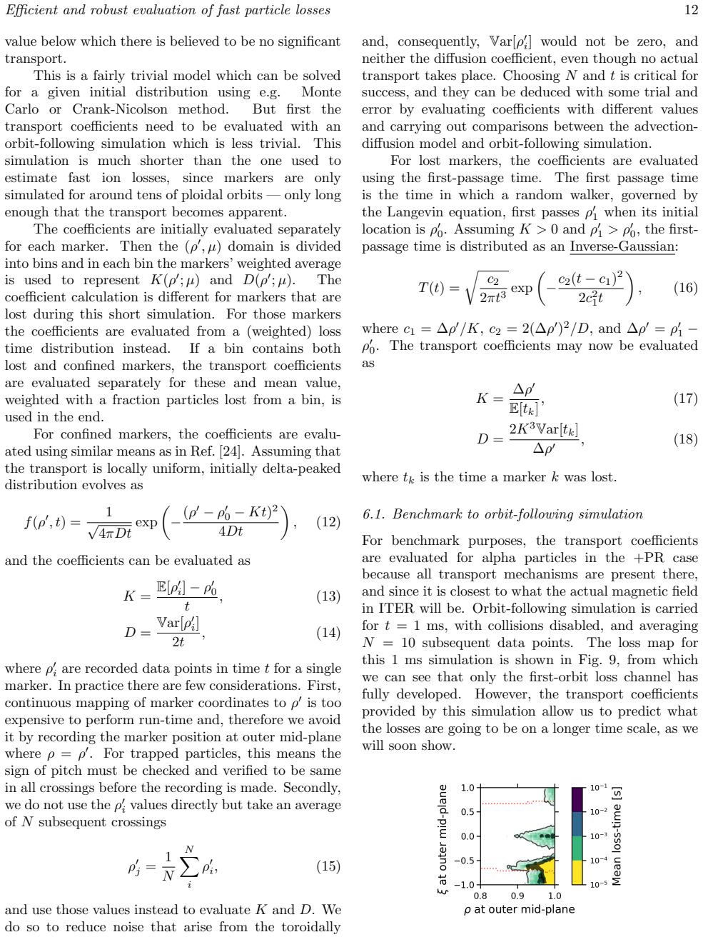
- [Section 6, Eqs. (13)-(15)] The transport coefficients K and D are evaluated as finite-time estimates from a single 1 ms collisionless simulation with N=10 OMP-crossing averaging, and the manuscript states that choosing N and t is critical and that they were deduced with trial and error. No sensitivity analysis with respect to t, N, or the reflecting boundary location is reported. This is load-bearing because Eqs. (11)-(14) yield genuine Fokker-Planck coefficients only if K and D are independent of the estimation window; if they are not, the advection-diffusion model is a tuned fitting procedure rather than a physics-based transport model. The point is reinforced by Figure 9, which shows that after 1 ms only the first-orbit loss channel is fully developed while the stochastic-ripple, stochastic-field-line, and perturbed-banana channels contribute only through small sub-threshold displacements. The authors should show that K and D converge as t and N are varied, and ideally that the model reproduces the time history of losses, not just the final loss map.
- [Section 6.1 and Fig. 10; Section 6.2 and Fig. 11] The benchmark accuracy is quantified only through total lost power: the advection-diffusion model gives 2.46 MW versus 1.79 MW from the collisionless orbit-following simulation (a 37% overestimate), and in the short-time comparison 1.42 MW versus 1.22 MW (a 16% overestimate). In the ECC phase scan the model systematically underestimates the losses in exactly the high-loss cases that a design scan is intended to identify. Since the stated purpose of the model is to find interesting regions in parameter space and provide rough estimates, the paper should report a quantitative accuracy metric for the scan, such as rank correlation or per-case relative error, and demonstrate that the high-loss cases are not systematically missed or suppressed. As it stands, the claim that the model is suitable for fast parameter scans is supported mainly by the qualitative visual agreement of the loss contours.
- [Section 6.1 and Section 6.2] The transport coefficients are evaluated with the same orbit-following code (ASCOT5) that provides the reference losses, so the advection-diffusion benchmarks test only whether the reduced 1D model can reproduce the output of the same code; they do not test the physical fidelity of the coefficients. The genuine 1 ms-to-100 ms time extrapolation is a meaningful test of time-independence, but it remains a self-consistency check. To support the physical claim that collisionless fast-ion transport is advection-diffusive, the authors should compare the inferred coefficients with the analytic expectations for at least one channel, e.g., the stochastic-ripple diffusion coefficient of Eq. (7) or the stochastic-field-line estimate of Eq. (9), or benchmark against an independent orbit-following implementation.
minor comments (6)
- [Eq. (2)] The definition of the magnetic moment appears to be missing the factor m/2 and should be clarified; as written, mu has units of m^2/s^2 rather than the usual J/T.
- [Section 5.1] The text says the stochastic-ripple diffusion coefficient is projected using Eq. (9), but Eq. (9) is the stochastic-field-line diffusion coefficient; the ripple diffusion coefficient is Eq. (7).
- [Section 6, first paragraph] The sentence 'comes from Ref. where this was shown' has an empty citation; the reference number is missing.
- [Eq. (16)] The inverse-Gaussian first-passage-time formula is rendered ambiguously: the denominator in the exponential should be 2 c_1^2 t, and c_1, c_2 should be defined more explicitly. The current notation is hard to parse.
- [Section 6, coefficient evaluation paragraph] The averaging in Eq. (15) is not fully specified: it should be stated explicitly that the rho'_j are OMP-crossing averages for a single marker and that the final K and D are weighted averages over markers in each (rho',mu) bin, including how the weights are defined.
- [Throughout] There are numerous typos and misspellings, including 'leves' for 'levels', 'quaranteed' for 'guaranteed', 'ploidal' for 'poloidal', 'extent' for 'extend', and 'absent' for 'absence'. A careful proofreading pass is needed.
Circularity Check
No significant circularity: the advection-diffusion prediction is a long-time extrapolation from short-trajectory statistics, and the ECC phase scan is out-of-sample.
full rationale
The central claim in Section 6 is that short 1 ms collisionless orbit-following statistics yield Fokker-Planck coefficients K and D (Eqs. 13-14) which, when inserted into Eq. (11), reproduce the 100 ms loss map and enable fast ECC-phase scans. This is not circular by construction: the final 100 ms loss fractions are not used to evaluate K and D; the coefficients come from displacement moments and first-passage times of the short simulation. The benchmark in Section 6.1 reports a genuine mismatch (2.46 MW model vs 1.79 MW collisionless orbit-following), and the 64-case scan in Section 6.2 systematically underpredicts high-loss cases while reproducing only the overall shape. Those discrepancies are exactly what an out-of-sample test should show and are not consistent with a forced fit. The sentence that choosing N and t 'can be deduced with some trial and error by evaluating coefficients with different values and carrying out comparisons' discloses hyperparameter tuning of the smoothing/averaging window; this is a robustness concern, not a circular reduction, because the predicted scan is not statistically forced by those hyperparameters. The magnetic-field-based loss projection in Section 5.1 provides an independent cross-check for one case (1.24 MW vs 1.18 MW) without using the advection-diffusion coefficients. Self-citations, mainly to Ref. [7] for loss-map concepts and perturbed-banana transport, are not load-bearing for the 100x speedup or scan suitability claims. The dangling citation 'Ref. where this was shown to be true for runaway electrons' is an editorial omission, not a circular dependency. Overall, the derivation is self-contained as a reduced-model validation: a short-time surrogate is built and then tested against a full simulation at long times and across new configurations.
Assumptions & free parameters
free parameters (3)
- Averaging window N and evaluation time t for transport coefficients =
N = 10 subsequent OMP crossings, t = 1 ms
- Reflecting boundary location in rho-prime =
Not specified; 'or at rho-prime value below which there is believed to be no significant transport'
- Reduced-field temperature and density assumptions =
T = 10 keV, n = 0.5 n_G (Greenwald density)
assumptions (4)
- domain assumption P_phi can be used to categorize particle orbit topology even when it is not conserved in non-axisymmetric fields.
- ad hoc to paper Collisionless fast ion transport can be represented as a 1D Fokker-Planck process in rho-prime with mu and E as parameters.
- domain assumption Collisions can be neglected for alpha particle losses on the relevant 100 ms timescale.
- standard math Standard Fokker-Planck and inverse Gaussian first-passage time statistics.
Cite this review
Pith. "Pith review of Efficient and robust evaluation of fast particle losses in non-axisymmetric tokamak plasmas." pith.science (2026). https://pith.science/paper/EBEHQIAW
@misc{pith2026190802494,
  author       = {Pith},
  title        = {Pith review of: Efficient and robust evaluation of fast particle losses in non-axisymmetric tokamak plasmas},
  year         = {2026},
  howpublished = {\url{https://pith.science/paper/EBEHQIAW}},
  note         = {Machine review of arXiv:1908.02494}
}
read the original abstract
We present various techniques that make orbit-following Monte Carlo simulations faster and more reliable when assessing collisionless fast particle losses due to magnetic field perturbations. These techniques are based on identifying various loss channels in constants of motion space using the so-called loss maps. We demonstrate that this allows one to attribute losses quantitatively to different transport mechanisms, increase signal-to-noise ratio when estimating FILD signal and peak power loads, and connect magnetic field structure directly to fast particle losses. Furthermore, we show that collisionless fast particle transport can be treated as an advection-diffusion process where the transport coefficients can be evaluated with the orbit-following method. Applying these techniques has the potential to make orbit-following simulations faster to perform, or to avoid them completely, while making the results more reliable as they become more clearly connected to underlying physics. We demonstrate these techniques for ITER by showing how alpha particle losses are affected by various magnetic field perturbations, estimating ICRH losses in reduced field scenarios, and performing a scan on alpha particle losses as a function of ELM control coil current phases.
Figures

Figures from the paper (9 more)

Reference graph
Works this paper leans on
-
[1]
Varje J, Asunta O, Cavinato M, Gagliardi M, Hirvijoki E, Koskela T, Kurki-Suonio T, Liu Y, Parail V, Saibene G, Sipil¨ a S, Snicker A, S¨ arkim¨ aki K and¨Ak¨ aslompolo S 2016 Nuclear Fusion 56 046014 doi: 10.1088/0029- 5515/56/4/046014
doi:10.1088/0029- 2016
-
[2]
Varje J, S¨ arkim¨ aki K, Kontula J, Ollus P, Kurki-Suonio T, Snicker A, Hirvijoki E and ¨Ak¨ aslompolo S In press Journal
-
[3]
39th EPS Conference on Plasma Physics p P5 URL http://ocs.ciemat.es/ epsicpp2012pap/pdf/P5.088.pdf
Akers R, Verwichte E, Martin T, Pinches S and Lake R 2012 GPGPU Monte Carlo calculation of gyro- phase resolved fast ion and n-state resolved neutral deuterium distributions Proc. 39th EPS Conference on Plasma Physics p P5 URL http://ocs.ciemat.es/ epsicpp2012pap/pdf/P5.088.pdf
work page 2012
-
[4]
26th IAEA Fusion Energy Conference pp TH/4–1 URL https://nucleus
Akers R, Colling B, Hess J, Liu Y, Turner A, ¨Ak¨ aslompolo S, Varje J, S¨ arkim¨ aki K, Pinches S and Singh M 2018 High fidelity simulations of fast ion power flux driven by 3d field perturbations on iter Proc. 26th IAEA Fusion Energy Conference pp TH/4–1 URL https://nucleus. iaea.org/sites/fusionportal/Shared%20Documents/ FEC%202016/fec2016-preprints/prepr...
work page 2018
-
[5]
Kurki-Suonio T, Asunta O, Hellsten T, Hyn¨ onen V, Johnson T, Koskela T, L¨ onnroth J, Parail V, Roccella M, Saibene G, Salmi A and Sipil¨ a S 2009Nuclear Fusion 49 095001 doi: 10.1088/0029-5515/49/9/095001
-
[6]
Tani K, Shinohara K, Oikawa T, Tsutsui H, Miyamoto S, Kusama Y and Sugie T 2011 Nuclear Fusion 52 013012 doi: 10.1088/0029-5515/52/1/013012
-
[7]
S¨ arkim¨ aki K, Varje J, B´ ecoulet M, Liu Y and Kurki-Suonio T 2018 Nuclear Fusion 58 076021 doi: 10.1088/1741- 4326/aac393
doi:10.1088/1741- 2018
-
[8]
White R B, Goldston R J, Redi M H and Budny R V 1996 Physics of Plasmas 3 3043–3054 doi: 10.1063/1.871641
Show all 24 references
-
[9]
Hsu C T and Sigmar D J 1992 Physics of Fluids B: Plasma Physics 4 1492–1505 doi: 10.1063/1.860060
1992 doi
-
[10]
Goldston R J, White R B and Boozer A H 1981 Physical Review Letters 47 647–649 doi: 10.1103/phys- revlett.47.647
1981 doi
-
[11]
Tobita K, Tani K, Neyatani Y, van Blokland A A E, Miura S, Fujita T, Takeuchi H, Nishitani T, Matsuoka M and Takechi S 1992 Physical Review Letters 69 3060–3063 doi: 10.1103/physrevlett.69.3060
1992 doi
-
[12]
Rechester A B and Rosenbluth M N 1978 Physical Review Letters 40 38–41 doi: 10.1103/physrevlett.40.38
1978 doi
-
[13]
¨Ak¨ aslompolo S, Kurki-Suonio T, Asunta O, Cavinato M, Gagliardi M, Hirvijoki E, Saibene G, Sipil¨ a S, Snicker A, S¨ arkim¨ aki K and Varje J 2015Nuclear Fusion 55 093010 doi: 10.1088/0029-5515/55/9/093010
-
[14]
Kurki-Suonio T, S¨ arkim¨ aki K,¨Ak¨ aslompolo S, Varje J, Liu Y, Sipil¨ a S, Asunta O, Hirvijoki E, Snicker A, Ter¨ av¨ a J, Cavinato M, Gagliardi M, Parail V and Saibene G 2016 Plasma Physics and Controlled Fusion 59 014013 doi: 10.1088/0741-3335/59/1/014013
2016 doi
-
[15]
Kurki-Suonio T, ¨Ak¨ aslompolo S, S¨ arkim¨ aki K, Varje J, Asunta O, Cavinato M, Gagliardi M, Hirvijoki E, Parail V, Saibene G, Sipil¨ a S and Snicker A 2016Nuclear Fusion 56 112024 doi: 10.1088/0029-5515/56/11/112024
-
[16]
Parail V, Albanese R, Ambrosino R, Artaud J F, Besseghir K, Cavinato M, Corrigan G, Garcia J, Garzotti L, Gribov Y, Imbeaux F, Koechl F, Labate C, Lister J, Litaudon X, Loarte A, Maget P, Mattei M, McDonald D, Nardon E, Saibene G, Sartori R and Urban J 2013 Nuclear Fusion 53 1...
2013 doi
-
[17]
¨Ak¨ aslompolo S, Asunta O, Bergmans T, Gagliardi M, Galabert J, Hirvijoki E, Kurki-Suonio T, Sipil¨ a S, Snicker A and S¨ arkim¨ aki K 2015Fusion Engineering and Design 98-99 1039–1043 doi: 10.1016/j.fusengdes.2015.05.038
2015 doi
-
[18]
Liu Y, ¨Ak¨ aslompolo S, Cavinato M, Koechl F, Kurki- Suonio T, Li L, Parail V, Saibene G, S¨ arkim¨ aki K, Sipil¨ a S and Varje J 2016Nuclear Fusion 56 066001 doi: 10.1088/0029-5515/56/6/066001
-
[19]
Illustration of the toroidal magnetic field ripple in different magnetic configurations
Evans T, Orlov D, Wingen A, Wu W, Loarte A, Casper Efficient and robust evaluation of fast particle losses 16 a) Ripple at OMP separatrix b) Ripple well c) Ripple magnitude TF +FI +TBM Figure A1. Illustration of the toroidal magnetic field ripple in different magnetic configuration...
2013
-
[20]
2018 ITER Research Plan within the Staged Approach (Level III - Provisional Version) Tech. rep. ITER Organi- zation URL https://www.iter.org/technical-reports
2018
-
[21]
Shinohara K, Oikawa T, Urano H, Oyama N, Lon- nroth J, Saibene G, Parail V and Kamada Y 2009 Fusion Engineering and Design 84 24–32 doi: 10.1016/j.fusengdes.2008.08.040
2009 doi
-
[22]
Kurki-Suonio T, S¨ arkim¨ aki K, Snicker S, Schneider M, Polevoi A and Mitteau R 2018 Beam Ion Performance and Power Loads in the ITER Pre-Fusion Power Operating Scenarios (PFPO) with Reduced Field and Current 27th IAEA Fusion Energy Conference URL https://conferences.iaea.org...
2018
-
[23]
Schneider M, POLEVOI A, Kim S, Loarte A, ARTAUD J, Beaumont B, Bilato R, Boilson D, Campbell D, Dumortier P et al. 2018
2018
-
[24]
Illustration of the toroidal magnetic field ripple in reduced field scenarios
Boozer A H 1981 Physics of Fluids 24 851 doi: 10.1063/1.863445 Efficient and robust evaluation of fast particle losses 18 a) Ripple at OMP separatrix b) Ripple well c) Ripple magnitude Full Half Third Figure A3. Illustration of the toroidal magnetic field ripple in reduced field s...
1981 doi
Reviewed August 14, 2026 · model on record in the stance chip above.
Discussion (0). Continue with ORCID to comment.