Bayesian estimation of the functional spatial lag model

Alassane Aw; Emmanuel Nicolas Cabral

REVIEW 4 major objections 5 minor 30 references

Bayesian estimation of the functional spatial lag model

T0 review · 4 major / 5 minor · reviewed 2026-08-14 · deepseek-v4-flash

Challenge this review Re-run · record.json Download PDF Read on arXiv ↗ Review JSON

Pith's one-line read The paper proposes a Metropolis-within-Gibbs estimator for the functional spatial lag model and argues, from simulations and a Senegalese application, that it outperforms truncated maximum likelihood.

desk verdict Correct Bayesian machinery for a modest extension, but the simulation evidence for the paper's main claim doesn't hold up—the BIC numbers are internally inconsistent. read the letter →

arxiv 1908.02739 v1 pith:YCW5EMXO submitted 2019-08-07 stat.ME

Alassane Aw , Emmanuel Nicolas Cabral This is my paper · ORCID

classification stat.ME MSC 62F1562H1162P2060J2262-07

keywords functionalspatiallagmodelBayesianestimationMetropolis-within-GibbsMCMCdataanalysisautoregressionSenegalunemployment

verification ladder T0 review T1 audit T2 compute T3 formal

The pith

A machine-rendered reading of the paper's core claim, the machinery that carries it, and where it could break.

The reading

This paper proposes a Bayesian way to estimate the functional spatial lag model, in which each spatial unit has a curve-valued predictor and its response depends on neighboring responses through a spatial weight matrix. The authors construct a Metropolis-within-Gibbs sampler: the slope coefficients and the error variance are drawn from their closed-form conditional distributions, while the spatial autoregressive parameter is updated with a Metropolis step using a normal or uniform proposal. Simulations over the 121 communes of Senegal are used to compare the sampler to truncated maximum likelihood, and the paper's stated finding is that the Bayesian estimates are better, with lower BIC values in the simulated settings. The method is then applied to explain unemployment rates in 45 Senegalese departments using illiteracy-rate curves, where the Bayesian estimates again come out ahead in the paper's comparison.

What carries the argument

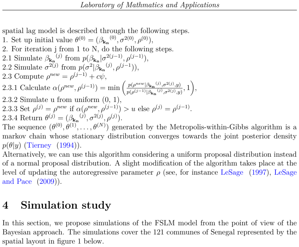
The central mechanism is the truncated basis expansion that turns the infinite-dimensional functional term into a finite design matrix. Writing $X_i(t)=\sum_{j=1}^\infty z_{ij}\varphi_j(t)$ and $\gamma(t)=\sum_{j=1}^\infty \beta_j\varphi_j(t)$ in an orthonormal basis, the inner product $\int_T X_i(t)\gamma(t)\,dt$ collapses to $\sum_{j=1}^{k_n} z_{ij}\beta_j$ once the tail is declared negligible. That reduction converts the functional spatial lag model into the matrix equation $y=\rho Wy+Z_{k_n}\beta_{k_n}+\epsilon$, after which the Bayesian machinery operates on a finite parameter vector. The load-bearing identity is therefore the basis expansion plus truncation, and the sampler's efficiency comes from the conjugate forms it induces for $\beta$ and $\sigma^2$.

What would settle it

Run the same Metropolis-within-Gibbs sampler on simulated data where the true functional coefficient has substantial components beyond the chosen truncation order $k_n$, or re-fit the Senegal data after changing the smoothing basis and the truncation order; if the posterior means of $\beta$ shift with the truncation and the BIC advantage over maximum likelihood disappears, the superiority claim is not general.

Watch

Extended reading notes

Core claim

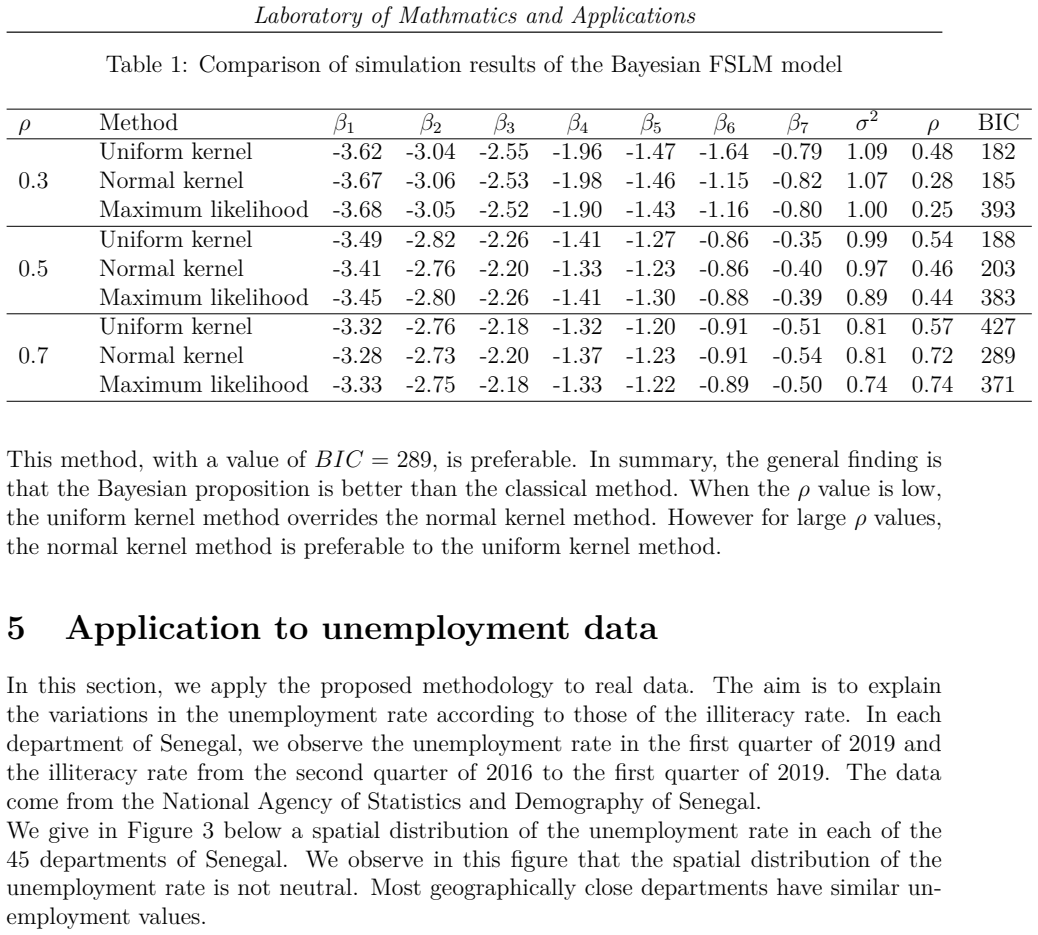
On its own terms, the paper establishes that Bayesian estimation of the functional spatial lag model is feasible and preferable to the frequentist baseline. With normal, inverse-gamma, and uniform priors on $\beta$, $\sigma^2$, and $\rho$, the posterior yields a Gibbs update for $\beta|\sigma^2,\rho$ that is multivariate normal with mean $(Z_{k_n}^T Z_{k_n} + \sigma^2\Sigma_{k_n}^{-1})^{-1}(Z_{k_n}^T A y + \sigma^2\Sigma_{k_n}^{-1} m_{k_n})$ and covariance $(Z_{k_n}^T Z_{k_n} + \sigma^2\Sigma_{k_n}^{-1})^{-1}$, and an inverse-gamma update for $\sigma^2|\beta,\rho$ with shape $n/2 + a$ and scale $((Ay - Z\beta)^T(Ay - Z\beta) + 2b)/2$; $\rho$ has no recognizable conditional form and is sampled by Metropolis-Hastings with an acceptance ratio involving $|I_n - \rho W|$. The paper claims that in simulations the sampler tracks the true $\rho$ across values 0.3, 0.5, and 0.7, and that BIC favors one Bayesian kernel over maximum likelihood in every scenario, supporting the conclusion that Bayesian estimation gives better results than frequentist estimation.

Load-bearing premise

The load-bearing premise is that the curves entering the model are the true curves: after smoothing noisy discrete observations with a 7 B-spline basis and truncating the basis expansion at $k_n$, the omitted tail is negligible, so the Bayesian posterior means are centered on the right quantities.

Editorial extensions

If this is right

For any dataset of functions observed over neighboring areas, the paper's sampler supplies posterior draws for the slope function, the error variance, and the spatial dependence parameter, not just point estimates.
Because the $\beta$ and $\sigma^2$ updates are standard conjugate draws, the per-iteration cost is essentially that of a Gaussian linear model, and only the $\rho$ step needs tuning.
The simulation comparisons imply that within-sample fit criteria such as BIC can prefer the Bayesian estimator over truncated maximum likelihood, giving practitioners a practical model-selection signal.
The Senegal application provides a template for regressing an areal economic outcome on curve-valued sociodemographic predictors, which may transfer to other administrative geographies.

Reading between the lines

Editorial extensions of the paper, not claims the author makes directly.

Because the curves are smoothed before estimation and treated as fixed, the reported posterior intervals do not account for smoothing or truncation error; a fully Bayesian treatment that puts a prior on the basis or truncation order would widen the uncertainty.
The closed-form updates for $\beta$ and $\sigma^2$ only depend on the spatial structure through $A = I - \rho W$, so the same template should extend to spatial error models or higher-order lags without a new derivation.
The paper's 'better' verdict rests on BIC and point recovery in a few simulation scenarios; comparing predictive performance on held-out departments would test whether the Bayesian advantage persists out of sample.

Share X Bluesky LinkedIn Reddit HN

Signed reviews

No signed human review yet.

Editorial analysis

A structured set of objections, weighed in public.

Desk editor's note, referee report, and a circularity audit.

Desk Editor's Note

read the letter

Dear colleague,

Here's my read of the Bayesian FSLM paper. The genuinely useful part is the derivation: a Metropolis-within-Gibbs sampler for the functional spatial lag model, with full conditionals for beta and sigma-squared in closed form and a random-walk MH step for rho. The algebra checks out—the Jacobian |I - ρW| in Eq. (10) is right, and Eqs. (13)–(14) are standard conjugate updates. This is a legitimate extension of LeSage and Pace's spatial econometrics machinery to functional covariates, and the paper correctly cites the relevant predecessors (Ahmed et al. 2017, Pineda-Rios et al. 2019).

The soft spot is exactly where the stress-test note lands: the empirical comparison. Section 6 claims Bayesian estimation gives better results than frequentist estimation, but the evidence for that is Table 1's BIC columns. No BIC formula is given, and the numbers contradict the likelihood in Eq. (10). Under the standard BIC with the same penalty and the same likelihood, the MLE has the largest log-likelihood among point estimates, so its BIC cannot be larger than the BIC at Bayesian point estimates. Table 1 reports ML BIC 393 versus uniform-kernel BIC 182 for ρ=0.3—a gap that would require the Bayesian point to have a log-likelihood about 105 units higher than the MLE. Either the "maximum likelihood" column isn't a converged MLE, or the Bayesian columns use a different criterion (marginal likelihood, DIC, or a different penalty). Either way, the table doesn't support the superiority claim.

There are smaller reporting gaps: one run per scenario, no Monte Carlo repetitions or error bars, no prior hyperparameters, no chain length or burn-in, no acceptance rates for the MH step in the simulation. The treatment of the functional covariate as known after B-spline smoothing is also underexplored, though that bias would affect both estimators similarly.

None of this breaks the derivation. The method is standard, the presentation is clear, and the reporting gaps are fixable. But the paper's headline finding is currently unsupported, and I wouldn't accept it in this state.

Who's it for? People working on spatial econometrics with functional data, who want a ready-to-implement Bayesian sampler. It's a useful toolbox addition, not a breakthrough. I'd send it to a referee—the core is sound—but I'd expect the referee to send it back for major revision on the simulations.

In short: worth engaging with, but the authors need to redo the simulation section and state their BIC.

Best,

Referee Report

4 major / 5 minor

Summary. The paper proposes a Bayesian MCMC estimator for the functional spatial lag model (FSLM), which extends the spatial lag model to functional covariates. The model is y = ρWy + Z β + ε, with β given a normal prior, σ² an inverse-gamma prior, and ρ a uniform prior. The authors derive the likelihood with Jacobian |I − ρW| (Eq. 10) and the full conditionals for β and σ² (Eqs. 13 and 14), then implement a Metropolis-within-Gibbs sampler with a random-walk proposal for ρ. Simulation experiments using 121 Senegalese communes compare the Bayesian estimator (with uniform and normal proposal kernels) against the maximum likelihood estimator of Ahmed et al. (2017), and an application relates unemployment to illiteracy curves across 45 departments. The central claim, stated in Section 6, is that Bayesian estimation gives better results than frequentist estimation, based largely on BIC values in Tables 1 and 2.

Significance. If the empirical comparison were valid, the paper would provide a useful Bayesian alternative for spatially dependent functional data. The theoretical core is essentially correct: the likelihood derivation in Eq. (10) properly includes the Jacobian, and the full conditionals in Eqs. (13) and (14) are algebraically sound. The Metropolis-within-Gibbs algorithm is standard and the application to real data is a useful illustration. However, the advertised conclusion of superiority over maximum likelihood rests on a flawed comparison metric (BIC) and a single simulation run. These issues, rather than the mathematical derivation, are the load-bearing weakness. The paper would need a substantially reworked simulation study and a properly specified model-comparison criterion before its conclusions could be accepted.

major comments (4)

[§4, Table 1 and §5, Table 2] The BIC comparison is internally inconsistent with maximum likelihood. Under the likelihood in Eq. (10) and any standard BIC with the same penalty term, the BIC evaluated at the maximum likelihood estimate must be less than or equal to the BIC evaluated at any other point estimate, because the MLE maximizes the log-likelihood by definition. Yet Table 1 reports, for ρ=0.3, ML BIC=393 and uniform-kernel Bayesian BIC=182, a gap that implies a log-likelihood difference of about 105 against the MLE. This is impossible unless the ML estimates are not converged, or the BIC values are computed with different likelihoods or penalties (for example, a marginal likelihood or DIC-type quantity in the Bayesian rows). No BIC formula is provided in the manuscript. Consequently, Tables 1 and 2 do not support the conclusion in Section 6 that the Bayesian method gives better results; the comparison metric must be specified and applied symmetrically.
[§4] The simulation study consists of a single replication for each value of ρ. Table 1 reports only point estimates with no Monte Carlo repetitions, no standard errors, no biases, and no RMSE. With a single data set, any observed ranking of the three methods can be entirely due to sampling variability. The claim in Section 6 that 'Bayesian estimation gives better results than frequentist estimation' is therefore not statistically supported. The simulation should be repeated over at least several hundred generated data sets, with Monte Carlo means, standard deviations, and error bars or boxplots.
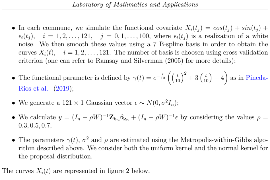
[§4 and §5] The treatment of the functional covariate is not fully justified. The curves are smoothed using a 7 B-spline basis chosen by cross-validation, and the truncation order is effectively k_n = 7, since the tables report β_1,...,β_7. However, no details are given on the truncation-order selection procedure, and no sensitivity analysis is reported. If the chosen basis dimension or truncation order is misspecified, the posterior means in Eqs. (13) and (14) are centered on the truncated approximation rather than on the true functional coefficient, affecting the interpretation of the estimated β and the spatial error variance. While this issue affects both Bayesian and maximum likelihood estimators, it is central to the validity of the model in the application, and should be addressed.
[§3.2 and Appendix] The MCMC implementation details are missing. The algorithm description does not specify the number of iterations, burn-in period, thinning, or starting values. The acceptance rates are reported for the real-data application (Table 2, column AR), but no definition or target range is given in the text. The trace plots in Figures 5 and 6 are described as 'stable', but no formal convergence diagnostics are provided. Without these details, the point estimates in Tables 1 and 2 cannot be assessed, and the Metropolis proposal tuning (constant c in Eq. (16)) is not documented.

minor comments (5)

[Throughout] The manuscript contains many typographical and grammatical errors (e.g., 'Mathmatics' in the affiliation, 'unkwon', 'choosen', 'derminant', 'eingenfunctions', 'intersted', 'corelated', 'wheter'). The paper needs careful proofreading.
[Section 2, Eq. (5)] The truncation remainder ∑_{j=k_n+1}^∞ z_{ij}β_j is asserted to be negligible with a reference to Müller and Stadtmüller (2005), but no rate condition or assumption on k_n is stated. A formal condition would clarify when the approximation is valid.
[Section 3.2, Eq. (17)] The acceptance probability in Eq. (17) omits the proposal density ratio; this is correct for a symmetric normal proposal, but when the alternative uniform proposal is used, the symmetry of the proposal near the boundary of the support [0,1] should be discussed. The handling of proposals that fall outside [0,1] is not described.
[Section 5] The Moran test is mentioned as confirming spatial autocorrelation, but no test statistic or p-value is reported. Also, the 'AR' column in Table 2 is not defined in the caption or text.
[Section 5, Table 2] For the maximum likelihood row, the 'AR' column is blank; the reader is left to infer that acceptance rate is only applicable to MCMC, but this should be stated explicitly.

Circularity Check

0 steps flagged · score 0.0 of 10

No circularity: the Bayesian full conditionals are derived from the stated likelihood and priors, and the empirical comparison with maximum likelihood is not an input to the derivation.

full rationale

The paper's derivation chain is self-contained. Equation (10) defines the likelihood from the functional spatial lag model in equation (7), and the stated normal, inverse-gamma, and uniform priors are combined with this likelihood in equation (11). The full conditional for sigma^2 in equation (13) follows algebraically from equation (12), and the full conditional for beta in equation (14) is the standard squared-completion result for a Gaussian likelihood with a Gaussian prior. The Metropolis-within-Gibbs algorithm then samples from these conditionals, with rho updated through the acceptance probability in equation (17). No parameter is fitted to a subset of data and then renamed as a prediction, and no load-bearing claim is justified by a self-citation: the cited Ahmed et al. (2017) result supplies the starting model, not the paper's Bayesian contribution. The simulation study generates data from the same model and compares posterior estimates with maximum likelihood, which is a conventional numerical check rather than a circular step. The reported BIC values in Tables 1 and 2 may be internally inconsistent with the stated likelihood, and the conclusion that Bayesian estimation 'gives better results' may therefore be empirically unsupported, but that is a correctness or validity concern, not a circularity of the derivation. Because the posterior distributions are derived from the model and priors without inserting the target result as an input, the circularity score is 0.

Assumptions & free parameters 4 free parameters · 6 assumptions · 0 invented entities

No invented entities are introduced. The model, priors, basis truncation, and smoothing choices are the main upstream inputs. The estimated parameters beta, sigma^2, and rho themselves are inferred from data and are not listed as free parameters.

free parameters (4)

Truncation order k_n = 7 (implied by beta_1,...,beta_7 in Tables 1 and 2)
Equation (5) truncates the infinite basis expansion; the choice of k_n controls the dimension of beta and is selected by cross-validation for smoothing, but no sensitivity analysis is provided.
B-spline basis dimension for functional covariates = 7
Used to smooth simulated and observed curves (Sections 4 and 5); chosen by cross-validation, but the criterion and its output are not shown.
Prior hyperparameters m_kn, Sigma_kn, a, b = not reported
Normal and inverse-gamma priors in Section 2 require values; they are never stated, so the posterior shown in Section 3 is not fully reproducible.
Random-walk tuning constant c = not reported
Equation (16) uses c to control the Metropolis proposal; the text only says acceptance should be between 40% and 60%.

assumptions (6)

domain assumption The functional covariate curves X_i(t) are fully observed after smoothing, with no measurement error propagated.
Sections 4 and 5 smooth discrete observations with B-splines and then treat curves as known in model (1); this is standard in FDA but can bias estimates.
domain assumption The truncation remainder sum_{j=k_n+1}^infinity z_ij beta_j is negligible.
Equation (5), required for model (6) to approximate model (1).
domain assumption Errors epsilon_i are independent and N(0, sigma^2).
Equation (1); no test for residual spatial correlation is reported beyond Moran's test on y.
domain assumption Spatial weights W are exogenous, row-standardized, and based on contiguity.
Equation (1) and Section 2; if W is misspecified, the estimate of rho is biased.
domain assumption Prior distributions for beta, sigma^2, and rho are independent.
Section 2 states 'we assume that all prior distributions are independent'; this is a standard simplifying assumption in Bayesian spatial econometrics.
domain assumption The spatial parameter rho lies in [0,1].
The uniform prior U[0,1] in Section 2 excludes negative spatial dependence, and the proposal in Eq. (16) can leave this interval without discussion.

how reviews work

0 comments

Cite this review

Pith. "Pith review of Bayesian estimation of the functional spatial lag model." pith.science (2026). https://pith.science/paper/YCW5EMXO

@misc{pith2026190802739,
  author       = {Pith},
  title        = {Pith review of: Bayesian estimation of the functional spatial lag model},
  year         = {2026},
  howpublished = {\url{https://pith.science/paper/YCW5EMXO}},
  note         = {Machine review of arXiv:1908.02739}
}

read the original abstract

The spatial lag model (SLM) has been widely studied in the literature for spatialised data modeling in various disciplines such as geography, economics, demography, regional sciences, etc. This is an extension of the classical linear model that takes into account the proximity of spatial units in modeling. The extension of the SLM model in the functional framework (the FSLM model) as well as its estimation by the truncated maximum likelihood technique have been proposed by \cite{Ahmed}. In this paper, we propose a Bayesian estimation of the FSLM model. The Bayesian MCMC technique is used as estimation methods of the parameters of the model. A simulation study is conducted in order to compare the results of the Bayesian estimation method with the truncated maximum likelihood method. As an illustration, the proposed Bayesian method is used to establish a relationship between the unemployment rate and the curves of illiteracy rate observed in the 45 departments of Senegal.

Figures

Figures reproduced from arXiv: 1908.02739 by the authors.

**Figure 2.** 121 curves Xi(t) obtained after smoothing the values Xi(tj ) by a 7 B-spline basis. We give in [PITH_FULL_IMAGE:figures/full_fig_p009_2.png] view at source ↗

**Figure 3.** Spatial distribution of the unemployment rate in Senegal. [PITH_FULL_IMAGE:figures/full_fig_p010_3.png] view at source ↗

Figures from the paper (3 more)

**Figure 4.** Figure 4: Curves of the rate of illiteracy of Senegal, obtained after expanding the data by [PITH_FULL_IMAGE:figures/full_fig_p011_4.png]

**Figure 5.** Figure 5: Markov chains produced by the Metropolis-within-Gibss algorithm with normal [PITH_FULL_IMAGE:figures/full_fig_p014_5.png]

**Figure 6.** Figure 6: Markov chains produced by the Metropolis-within-Gibss algorithm with uniform [PITH_FULL_IMAGE:figures/full_fig_p015_6.png]

Discussion (0). Continue with ORCID to comment.

Reference graph

Works this paper leans on

30 extracted references · 30 canonical work pages

[1]

Ahmed, M., Broze L., Dabo-Niang, S., Gharbi, Z. (2017). Functional Linear Spatial Autoregressive Models. Ramon Giraldo; Jorge Mateu. Geostatistical Functional Data Analysis: Theory and Methods, Wiley, 2017

work page 2017
[2]

Anselin, L. (1988). Spatial Econometrics: Methods and Models, Kluwer Academic Publishers, Dorddrecht

work page 1988
[3]

Caballero,W., Giraldo, R., Mateu, J. (2013). A universal kriging approach for spatial functional data. Stochastic Environmental Research and Risk Assessment, 27, 1553–1563

work page 2013
[4]

Casella, G., Georg, E. I. (1992). Explaining the Gibbs Sampler. The American Statistician, 46(3), 167–174

work page 1992
[5]

Cardot, H., Ferraty, F., Sarda, P. (1999). Functional linear model. Statistics and Probability Letters 45:11–22

work page 1999
[6]

Cardot, H., Ferraty, F., Mas, A., Sarda, P. (2003). Testing hypotheses in the functional linear model. Scandinavian Journal of Statistics, 30, 241–255

work page 2003
[7]

and Yao, F

Dabo-Niang, S. and Yao, F. (2007). Kernel regression estimation for continuous spatial processes. Mathematical Methods of Statistics, 16, 298–317

work page 2007
[8]

Delicado, P., Giraldo, R., Comas, C., Mateu, J. (2010). Statistics for spatial functional data: some recent contributions. Environmetrics, 21, 224–239

work page 2010

Show all 30 references

[9]

Doğan, O., Taşpınar, S. (2014). Spatial autoregressive models with unknown heteroskedasticity: A comparison of Bayesian and robust GMM approach. Regional Science and Urban Economics, 45, 1–21

2014
[10]

Gelman A., Carlin J., Stern H., Rubin D. (2013). Bayesian Data Analysis, 3rd edition. Chapman and Hall/CRC

2013
[11]

Gilks, W.R., Richardson, S., Spiegelhalter, D. (1995). Markov Chain Monte Carlo in Practice. Chapman and Hall/CRC

1995
[12]

Giraldo, R., Delicado, P., Mateu, J. (2011). Ordinary kriging for function-valued spatial data. Environmental and Ecological Statistics, 18, 411–426

2011
[13]

Hall P., Horowitz J.L. (2007). Methodology and convergence rates for functional linear regression. Annals of Statistics 35:70–91

2007
[14]

Hilgert, N., Mas, A., Verzelen, N. (2013). Minimax adaptive tests for the functional linear model. Annals of Statistics 41:838–869

2013
[15]

Horváth, L., Kokoszka, P. (2012). Inference for Functional Data with Applications. Springer

2012
[16]

Huang, T., Saporta, G., Wang, H., Wang, S. (2018). Spatial Functional Linear Model and its Estimation Method. arXiv:1811.00314 [stat.CO]

2018 arXiv
[17]

Jacques, J., Preda, C. (2014). Model-based clustering for multivariate functional data. Computational Statistics and Data Analysis, Elsevier, 2014, 71, pp.92-106

2014
[18]

Clustering for sparsely sampled functional data

James, G., Sugar, C., (2003). Clustering for sparsely sampled functional data. Journal of the American Statistical Association 98 (462), 397–408

2003
[19]

Bayesian Econometric Methods

Koop, G., Poirier, D.J., Tobias, J.L., (2007). Bayesian Econometric Methods. Cambridge University Press, New York, USA

2007
[20]

Lesage, J. P. (1997). Bayesian Estimation of Spatial Autoregressive Models. International Regional Science Review, 20(1-2), 113–129

1997
[21]

LeSage, J. P. and Pace R. K. (2009). Introduction to Spatial Econometrics. 1st Edn., CRC Press, ISBN-10:142006424X, pp: 374

2009
[22]

Müller, H.-G., Stadtmüller, U. (2005). Generalized functional linear models. Ann. Statist., 33 ,774–805

2005
[23]

Pineda-Rios, W., Giraldo, R., Porcu, E. (2019). Functional SAR models: With application to spatial econometrics. Spatial Statistics, 29, 145-159

2019
[24]

and Silverman, B

Ramsay, J.O. and Silverman, B. (2005). Functional Data Analysis. Springer

2005
[25]

O., Ramsay, T., Sangalli, L

Ramsay, J. O., Ramsay, T., Sangalli, L. M. (2011). Spatial Functional Data Analysis. Recent Advances in Functional Data Analysis and Related Topics, 269–275

2011
[26]

and Rosenthal, J.S

Roberts, G.O. and Rosenthal, J.S. (2004). General state space Markov chains and MCMC algorithms. Probability Surveys, 1, 20–71

2004
[27]

Tierney, L. (1994). Markov Chains for Exploring Posterior Distributions. The Annals of Statistics, 22, 1701-1728

1994
[28]

Zhang, J. (2013). Analysis of Variance for Functional Data. CRC Press

2013
[29]

A., Majewski, T., Czerniak, B

Zhang, L., Baladandayuthapani, V., Zhu, H., Baggerly, K. A., Majewski, T., Czerniak, B. A., Morris, J. S. (2016). Functional CAR models for large spatially correlated functional datasets. Journal of the American Statistical Association, 111, 772–786

2016
[30]

Zoglat, A. (2008). Functional analysis of variance. Applied Mathematical Sciences, 2, 1115–1129

2008

Pith tools

Reviewed August 14, 2026 · model on record in the stance chip above.

[1] [1]

Ahmed, M., Broze L., Dabo-Niang, S., Gharbi, Z. (2017). Functional Linear Spatial Autoregressive Models. Ramon Giraldo; Jorge Mateu. Geostatistical Functional Data Analysis: Theory and Methods, Wiley, 2017

work page 2017

[2] [2]

Anselin, L. (1988). Spatial Econometrics: Methods and Models, Kluwer Academic Publishers, Dorddrecht

work page 1988

[3] [3]

Caballero,W., Giraldo, R., Mateu, J. (2013). A universal kriging approach for spatial functional data. Stochastic Environmental Research and Risk Assessment, 27, 1553–1563

work page 2013

[4] [4]

Casella, G., Georg, E. I. (1992). Explaining the Gibbs Sampler. The American Statistician, 46(3), 167–174

work page 1992

[5] [5]

Cardot, H., Ferraty, F., Sarda, P. (1999). Functional linear model. Statistics and Probability Letters 45:11–22

work page 1999

[6] [6]

Cardot, H., Ferraty, F., Mas, A., Sarda, P. (2003). Testing hypotheses in the functional linear model. Scandinavian Journal of Statistics, 30, 241–255

work page 2003

[7] [7]

and Yao, F

Dabo-Niang, S. and Yao, F. (2007). Kernel regression estimation for continuous spatial processes. Mathematical Methods of Statistics, 16, 298–317

work page 2007

[8] [8]

Delicado, P., Giraldo, R., Comas, C., Mateu, J. (2010). Statistics for spatial functional data: some recent contributions. Environmetrics, 21, 224–239

work page 2010